|
1
2
3
4
5
6
7
8
9
10
11
12
13
14
15
16
17
18
19 |
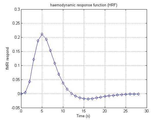
%%%%%%%%%%%%%%%%%%%%%%%%%%%%%%%%%clear all;clc;%%%%%%%%%%%%%%%%%%%%%%%%%%%%%%%%%%%%%%%%%%%%%%%%%%%%%%%%%%%%%%%%%%% haemodynamic response function: BOLD signal has stereotyped shape every% time a stimulus hits it. We usually use the spm_hrf.m in SPM toolbox to% produce HRF. Here, we use the 29
vector to represent HRF from 0
s to% 28
s. In this
simulation, we suppose TR=1
s.HRF = [0
0.004 0.043 0.121 0.188 0.211 0.193 0.153 0.108 0.069 0.038 0.016 0.001 -0.009 -0.015 -0.018 -0.019 -0.018 -0.015 -0.013 -0.010 -0.008 -0.006 -0.004 -0.003 -0.002 -0.001 -0.001 -0.001];% We will plot its shape with figure 1:figure(1)% here is the x-coordinatest = [0:28];plot(t,HRF,‘d-‘);grid on;xlabel(‘Time (s)‘);ylabel(‘fMRI respond‘);title(‘haemodynamic response function (HRF)‘); |
结果:
|
1
2
3
4
5
6
7
8
9
10
11
12
13
14
15
16
17
18
19
20
21
22
23 |
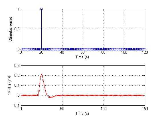
%%%%%%%%%%%%%%%%%%%%%%%%%%%%%%%%%%%%%%%%%%%%%%%%%%%%%%%%%%%%%%%%%%% Suppose that our scan for
120 s, we will have 120
point (because TR = 1% s). If a stimulus onset at t=20
s, we can use a vector to represent this% stimulation.onset_1 = [zeros(1,19) 1
zeros(1,100)];% i.e. the whole vector is maked with 19
zeros, a single 1, and then 100% zeros. As we have the stimulus onset vector and HRF we can convolve them.% In Matlab, the command to convolve two vectors is "conv":conv_1 = conv(HRF,onset_1);% Let‘s plot the result in figure 2figure(2);% This figure will have 2
rows of subplots.subplot(2,1,1);% "Stem"
is a good function for
showing discrete events:stem(onset_1);grid on;xlabel(‘Time (s)‘);ylabel(‘Stimulus onset‘);subplot(2,1,2);plot(conv_1,‘rx-‘);grid on;xlabel(‘Time (s)‘);ylabel(‘fMRI signal‘); |
结果:
|
1
2
3
4
5
6
7
8
9
10
11
12
13
14
15
16
17
18
19
20
21 |
%%%%%%%%%%%%%%%%%%%%%%%%%%%%%%%%%%%%%%%%%%%%%%%%%%%%%%%%%%%%%%%%%%% Usually, we have repeat a task many times in a run. If three stimulus % onsets at t=20, 50, 80
s, we also can use a vector to represent this% stimulation.onset_2 = [zeros(1,19) 1
zeros(1,29) 1
zeros(1,29) 1
zeros(1,20)];% Here we use the conv again:conv_2 = conv(HRF,onset_2);% Let‘s plot the result in figure 3figure(3);% This figure will have 2
rows of subplots.subplot(2,1,1);% "Stem"
is a good function for
showing discrete events:stem(onset_2);grid on;xlabel(‘Time (s)‘);ylabel(‘Stimulus onset‘);subplot(2,1,2);plot(conv_2,‘rx-‘);grid on;xlabel(‘Time (s)‘);ylabel(‘fMRI signal‘); |
结果: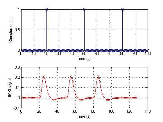
|
1
2
3
4
5
6
7
8
9
10
11
12
13
14
15
16
17 |
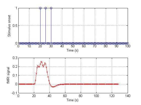
%%%%%%%%%%%%%%%%%%%%%%%%%%%%%%%%%%%%%%%%%%%%%%%%%%%%%%%%%%%%%%%%%%% Now let‘s think about the fast event design. In this
condition, we will% have many task during a short
time. If three stimulus onsets at t=20, 25,% 30
s:onset_3 = [zeros(1,19) 1
zeros(1,4) 1
zeros(1,4) 1
zeros(1,70)];conv_3 = conv(HRF,onset_3);figure(4);subplot(2,1,1);stem(onset_3);grid on;xlabel(‘Time (s)‘);ylabel(‘Stimulus onset‘);subplot(2,1,2);plot(conv_3,‘rx-‘);grid on;xlabel(‘Time (s)‘);ylabel(‘fMRI signal‘); |
结果:
|
1
2
3
4
5
6
7
8
9
10
11
12
13
14
15
16
17
18 |
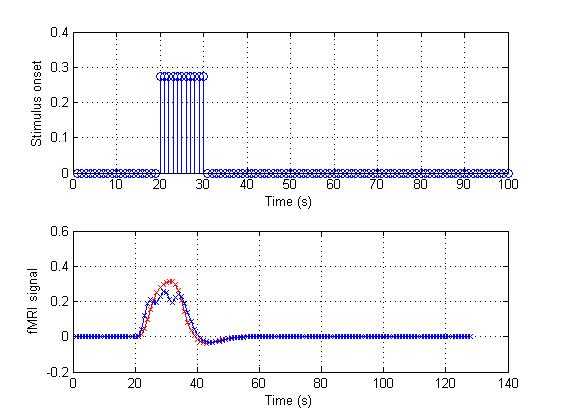
% The three events are so closed, the result signal is like a blocked% design. Such as:onset_4 = [zeros(1,19) ones(1,11) zeros(1,70)]*(3/11);conv_4 = conv(HRF,onset_4);figure(5);subplot(2,1,1);stem(onset_4);grid on;xlabel(‘Time (s)‘);ylabel(‘Stimulus onset‘);subplot(2,1,2);plot(conv_4,‘rx-‘);% We will compare the resulthold on; % plot more than one time on a figureplot(conv_3,‘bx-‘);grid on;xlabel(‘Time (s)‘);ylabel(‘fMRI signal‘); |
结果:
对于fmri的hrf血液动力学响应函数的一个很直观的解释-by 西南大学xulei教授,布布扣,bubuko.com
对于fmri的hrf血液动力学响应函数的一个很直观的解释-by 西南大学xulei教授
原文:http://www.cnblogs.com/haore147/p/3633515.html