matlab使用练习（6）

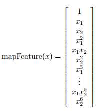
Regularized logistic regression : 

ex2_reg.m

%% =========== Part 1: Regularized Logistic Regression ============
% In this part, you are given a dataset with data points that are not
% linearly separable. However, you would still like to use logistic
% regression to classify the data points.
%
% To do so, you introduce more features to use -- in particular, you add
% polynomial features to our data matrix (similar to polynomial
% regression).
%

% Add Polynomial Features

% Note that mapFeature also adds a column of ones for us, so the intercept
% term is handled
X = mapFeature(X(:,1), X(:,2));  %调用下面的mapFeature.m文件中的mapFeature(X1,X2)函数

                                           %将只有x1,x2feature的map成一个有28个feature的6次的多项式 ,这样就能画出更复杂的decision boundary

                                            %  调用完后X变为118*28(118个example,28个属性，包括前面的1做为一列)的矩阵

% Initialize fitting parameters
initial_theta = zeros(size(X, 2), 1);    %initial_theta: 28*1

% Set regularization parameter lambda to 1  
lambda = 1;                                    %λ=1

% Compute and display initial cost and gradient for regularized logistic
% regression
[cost, grad] = costFunctionReg(initial_theta, X, y, lambda);

fprintf(‘Cost at initial theta (zeros): %f\n‘, cost);

fprintf(‘\nProgram paused. Press enter to continue.\n‘);
pause;

mapFeature.m

function out = mapFeature(X1, X2)
% MAPFEATURE Feature mapping function to polynomial features
%
% MAPFEATURE(X1, X2) maps the two input features
% to quadratic features used in the regularization exercise.
%
% Returns a new feature array with more features, comprising of
% X1, X2, X1.^2, X2.^2, X1*X2, X1*X2.^2, etc..
%
% Inputs X1, X2 must be the same size
%

degree = 6;       %map the features into all polynomial terms of x1 and x2 up to the sixth power

out = ones(size(X1(:,1)));
for i = 1:degree
for j = 0:i
out(:, end+1) = (X1.^(i-j)).*(X2.^j);
end
end

end

matlab使用练习（6）

原文：http://www.cnblogs.com/yan2015/p/4839617.html