前言
论文“Reducing the Dimensionality of Data with Neural Networks”是深度学习鼻祖hinton于2006年发表于《SCIENCE 》的论文,也是这篇论文揭开了深度学习的序幕。
笔记
摘要:高维数据可以通过一个多层神经网络把它编码成一个低维数据,从而重建这个高维数据,其中这个神经网络的中间层神经元数是较少的,可把这个神经网络叫做自动编码网络或自编码器(autoencoder)。梯度下降法可用来微调这个自动编码器的权值,但是只有在初始化权值较好时才能得到最优解,不然就容易陷入局部最优解。本文提供了一种有效的初始化权值算法,就是利用深度自动编码网络来学习得到初始权值。这一算法比用主成份分析(PCA)来对数据进行降维更好更有效。
内容:
降维在分类、可视化、通信、高维数据的存储等方面都非常有促进作用。一个简单且广泛应用的方法就是PCA降维,它通过寻找数据中的最大变化方向,然后把每个数据都投影到这些方向构成的坐标系中,并表示出来。本文提出了一种PCA的非线性泛化算法,该算法用一个自适应的多层自动编码网络来把高维数据编码为一个低维数据,同时用一个类似的解码网络来把这个低维数据重构为原高维数据。
首先,对这两个网络的权值进行随机初始化,然后通过最小化重构项和原始数据之间的误差对权值进行训练。误差的偏导数通过后向传播得到梯度,也就是把误差偏导数先通过解码网络,再通过编码网络进行传播。整个系统叫做自编码器,具体见图1。
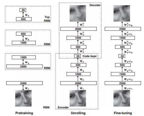
图1.预训练,就是训练一系列的RBM,每个RBM只有一层特征检测器。前一个RBM学习的特征作为下一个RBM的输入。预训练完成后把RBM展开得到一个深层自动编码网络,然后把误差的偏导数后向传播,用来对这个网络进行微调。
最优化有多层隐藏层(2-4层)的非线性自编码器的权值比较困难。因为如果权值初始值较大时,自编码器非常容易陷入局部最优解;如果权值初始值较小时,前几层的梯度下降是非常小的,权值更新就非常慢,这样就必须增加自编码器的隐藏层数,不然就训练不出最优值。如果初始权值比较接近最优解,那么就能能过梯度下降法很快训练得到最优解,但是通过一次学习一层特征的算法来找出这样的初始权值非常困难。“预训练”可以很好地解决这一问题,通过“预训练”可以得到比较接近最优解的初始权值。虽然本文中的“预训练”过程是用的二值数据,但是推广到其他真实的数据也是可以的,并且证明是有效的。
一个二值向量(如:图像)可以通过一个2层网络(即:RBM)来重构,在RBM(文献[5][6])中,通过对称加权连接把随机二值像素点和随机二值特征检测器联系起来。那些像素点相当于RBM的可视化单元,因为它们的状态是可见的;那些特征检测器相当于隐藏单元。可视单元和隐藏单元的联合系统(v,h)之间的能量(文献[7])表示为:
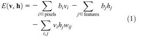
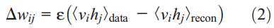
其中,vi和hj分别是第i个可视层单元和第j个隐藏层单元的状态,bi和bj是偏置项,wji是权值。这个网络通过这个能量函数得到每个可能图像的概率,具体解释见文献[8]。神经元的输入输出关系是;sigmoid函数。给定一张输入图像(暂时是以二值图像为例),我们可以通过调整网络的权值和偏置值使得网络对该输入图像的能量最低。权值更新公式如下:
单层的二值网络不足以模拟大量的数据集,因此一般采用多层网络,即把第一层网络的输出作为第二层网络的输入。并且每增加一个网络层,就会提高网络对输入数据重构的log下界概率值,且上层的网络能够提取出其下层网络更高阶的特征。
当网络的预训练过程完成后,我们需要把解码和编码部分重新拿回来展开构成整个网络,然后用真实的数据作为样本标签来微调网络的参数。
对于连续的数据,第一个RBM的隐藏层仍然是二值的,但是其可视化层单元是带高斯白噪声的线性单元。如果该噪声是单位方差,隐藏单元的更新规则仍然是一样的,第i个可视化层单元的更新规则是从一个高斯噪声中抽样,这个噪声的方差是单位方差,均值是 的平均值。
的平均值。
在实验中,每个RBM的可视层单元都有真实的[0,1]内激活值,对于高层RBM,其可视化层单元就是前一个RBM的隐藏层单元的激活概率,但是除了最上面一个RBM之外,其他的RBM的隐藏层单元都是随机的二值。最上面一个RBM的隐藏单元是一个随机实值状态,它是从单位方差噪声中抽样得到的,这个单位方差噪声的均值由RBM的可视单元决定。比起PCA,本算法较好地利用了连续变量。预训练和微调的细节见文献[8]。
接下来,做了一系列实验。
实验
实验基础说明
1.实验代码:http://www.cs.toronto.edu/~hinton/MatlabForSciencePaper.html
2.一些matlab函数
rem和mod:
参考资料取模(mod)与取余(rem)的区别——Matlab学习笔记
通常取模运算也叫取余运算,它们返回结果都是余数.rem和mod唯一的区别在于:
当x和y的正负号一样的时候,两个函数结果是等同的;当x和y的符号不同时,rem函数结果的符号和x的一样,而mod和y一样。这是由于这两个函数的生成机制不同,rem函数采用fix函数,而mod函数采用了floor函数(这两个函数是用来取整的,fix函数向0方向舍入,floor函数向无穷小方向舍入)。rem(x,y)命令返回的是x-n.*y,如果y不等于0,其中的n = fix(x./y),而mod(x,y)返回的是x-n.*y,当y不等于0时,n=floor(x./y)
3.函数说明
converter.m:
实现的功能是将样本集从.ubyte格式转换成.ascii格式,然后继续转换成.mat格式。
makebatches.m:
实现的是将原本的2维数据集变成3维的,因为分了多个批次,另外1维表示的是批次。
function [f, df] = CG_MNIST(VV,Dim,XX);
该函数实现的功能是计算网络代价函数值f,以及f对网络中各个参数值的偏导数df,权值和偏置值是同时处理。其中参数VV为网络中所有参数构成的列向量,参数Dim为每层网络的节点数构成的向量,XX为训练样本集合。f和df分别表示网络的代价函数和偏导函数值。
共轭梯度下降的优化函数形式为:
[X, fX, i] = minimize(X, f, length, P1, P2, P3, ... )
该函数时使用共轭梯度的方法来对参数X进行优化,所以X是网络的参数值,为一个列向量。f是一个函数的名称,它主要是用来计算网络中的代价函数以及代价函数对各个参数X的偏导函数,f的参数值分别为X,以及minimize函数后面的P1,P2,P3,…使用共轭梯度法进行优化的最大线性搜索长度为length。返回值X为找到的最优参数,fX为在此最优参数X下的代价函数,i为线性搜索的长度(即迭代的次数)。
实验步骤
1.加载数据集,并转换为.mat格式,即代码中的converter.m;
2.依次预训练4个rbm,并把前一个rbm的输入作为后一个rbm的输入,见rbm.m;
3.把4个rbm展开成图1中的“Unrolling”部分,计算该网络的代价函数及其对各权值的偏导数,见CG_MNIST.m;
4.利用共轭梯度下降法对代价函数进行优化,见minimize.m。
实验结果
Train squared error: 4.318
Test squared error: 4.520
代码
mnistdeepauto.m
% Version 1.000
%
% Code provided by Ruslan Salakhutdinov and Geoff Hinton
%
% Permission is granted for anyone to copy, use, modify, or distribute this
% program and accompanying programs and documents for any purpose, provided
% this copyright notice is retained and prominently displayed, along with
% a note saying that the original programs are available from our
% web page.
% The programs and documents are distributed without any warranty, express or
% implied.  As the programs were written for research purposes only, they have
% not been tested to the degree that would be advisable in any important
% application.  All use of these programs is entirely at the user‘s own risk.


% This program pretrains a deep autoencoder for MNIST dataset
% You can set the maximum number of epochs for pretraining each layer
% and you can set the architecture of the multilayer net.

clear all
close all

maxepoch=10; %最大迭代次数  In the Science paper we use maxepoch=50, but it works just fine.
numhid=1000; numpen=500; numpen2=250; numopen=30;

fprintf(1,‘Converting Raw files into Matlab format \n‘);
converter; % 把测试数据集和训练数据集转换为.mat格式

fprintf(1,‘Pretraining a deep autoencoder. \n‘);
fprintf(1,‘The Science paper used 50 epochs. This uses %3i \n‘, maxepoch);

makebatches;% 把数据集及其标签进行打包或分批,方便以后分批进行处理,因为数据太大了
[numcases numdims numbatches]=size(batchdata);%返回训练数据集的大小

fprintf(1,‘Pretraining Layer 1 with RBM: %d-%d \n‘,numdims,numhid);
restart=1;
rbm;             %预训练第1个rbm
hidrecbiases=hidbiases; % 第一个rbm的隐含层偏置项
save mnistvh vishid hidrecbiases visbiases;% 保存第1个rbm的权值、隐含层偏置项、可视化层偏置项,为mnistvh.mat

fprintf(1,‘\nPretraining Layer 2 with RBM: %d-%d \n‘,numhid,numpen);
batchdata=batchposhidprobs;% 第1个rbm中整个数据第一次正向传播时隐含层的输出概率,作为第2个rbm的输入数据
numhid=numpen;% 第2个rbm的隐含层神经元数
restart=1;
rbm;       %预训练第2个rbm
hidpen=vishid; penrecbiases=hidbiases; hidgenbiases=visbiases;
save mnisthp hidpen penrecbiases hidgenbiases;% 保存第2个rbm的权值、隐含层偏置项、可视化层偏置项,为mnisthp.mat

fprintf(1,‘\nPretraining Layer 3 with RBM: %d-%d \n‘,numpen,numpen2);
batchdata=batchposhidprobs;% 第2个rbm中整个数据第一次正向传播时隐含层的输出概率,作为第3个rbm的输入数据
numhid=numpen2;
restart=1;
rbm;       %预训练第3个rbm
hidpen2=vishid; penrecbiases2=hidbiases; hidgenbiases2=visbiases;
save mnisthp2 hidpen2 penrecbiases2 hidgenbiases2;% 保存第3个rbm的权值、隐含层偏置项、可视化层偏置项,为mnisthp2.mat

fprintf(1,‘\nPretraining Layer 4 with RBM: %d-%d \n‘,numpen2,numopen);
batchdata=batchposhidprobs;% 第3个rbm中整个数据第一次正向传播时隐含层的输出概率,作为第4个rbm的输入数据
numhid=numopen;
restart=1;
rbmhidlinear;
hidtop=vishid; toprecbiases=hidbiases; topgenbiases=visbiases;
save mnistpo hidtop toprecbiases topgenbiases;% 保存第4个rbm的权值、隐含层偏置项、可视化层偏置项,为mnistpo.mat

backprop;
converter.m
% Version 1.000
% % 作用:把测试数据集和训练数据集转换为.mat格式
% 最终得到的测试数据集:test(0~9).mat
% 最终得到的训练数据集:digit(0~9).mat
% Code provided by Ruslan Salakhutdinov and Geoff Hinton
%
% Permission is granted for anyone to copy, use, modify, or distribute this
% program and accompanying programs and documents for any purpose, provided
% this copyright notice is retained and prominently displayed, along with
% a note saying that the original programs are available from our
% web page.
% The programs and documents are distributed without any warranty, express or
% implied.  As the programs were written for research purposes only, they have
% not been tested to the degree that would be advisable in any important
% application.  All use of these programs is entirely at the user‘s own risk.

% This program reads raw MNIST files available at
% http://yann.lecun.com/exdb/mnist/
% and converts them to files in matlab format
% Before using this program you first need to download files:
% train-images-idx3-ubyte.gz train-labels-idx1-ubyte.gz
% t10k-images-idx3-ubyte.gz t10k-labels-idx1-ubyte.gz
% and gunzip them. You need to allocate some space for this.

% This program was originally written by Yee Whye Teh

%% 首先转换测试数据集的格式 Work with test files first
fprintf(1,‘You first need to download files:\n train-images-idx3-ubyte.gz\n train-labels-idx1-ubyte.gz\n t10k-images-idx3-ubyte.gz\n t10k-labels-idx1-ubyte.gz\n from http://yann.lecun.com/exdb/mnist/\n and gunzip them \n‘);

f = fopen(‘t10k-images.idx3-ubyte‘,‘r‘);
[a,count] = fread(f,4,‘int32‘);

g = fopen(‘t10k-labels.idx1-ubyte‘,‘r‘);
[l,count] = fread(g,2,‘int32‘);

fprintf(1,‘Starting to convert Test MNIST images (prints 10 dots) \n‘);
n = 1000;

Df = cell(1,10);
for d=0:9,
  Df{d+1} = fopen([‘test‘ num2str(d) ‘.ascii‘],‘w‘);
end;

for i=1:10,
  fprintf(‘.‘);
  rawimages = fread(f,28*28*n,‘uchar‘);
  rawlabels = fread(g,n,‘uchar‘);
  rawimages = reshape(rawimages,28*28,n);

  for j=1:n,
    fprintf(Df{rawlabels(j)+1},‘%3d ‘,rawimages(:,j));
    fprintf(Df{rawlabels(j)+1},‘\n‘);
  end;
end;

fprintf(1,‘\n‘);
for d=0:9,
  fclose(Df{d+1});
  D = load([‘test‘ num2str(d) ‘.ascii‘],‘-ascii‘);%这个test.ascii文件从哪来的?
  fprintf(‘%5d Digits of class %d\n‘,size(D,1),d);
  save([‘test‘ num2str(d) ‘.mat‘],‘D‘,‘-mat‘);
end;


%% 然后转换训练数据集的格式Work with trainig files second
f = fopen(‘train-images.idx3-ubyte‘,‘r‘);
[a,count] = fread(f,4,‘int32‘);

g = fopen(‘train-labels.idx1-ubyte‘,‘r‘);
[l,count] = fread(g,2,‘int32‘);

fprintf(1,‘Starting to convert Training MNIST images (prints 60 dots)\n‘);
n = 1000;

Df = cell(1,10);
for d=0:9,
  Df{d+1} = fopen([‘digit‘ num2str(d) ‘.ascii‘],‘w‘);
end;

for i=1:60,
  fprintf(‘.‘);
  rawimages = fread(f,28*28*n,‘uchar‘);
  rawlabels = fread(g,n,‘uchar‘);
  rawimages = reshape(rawimages,28*28,n);

  for j=1:n,
    fprintf(Df{rawlabels(j)+1},‘%3d ‘,rawimages(:,j));
    fprintf(Df{rawlabels(j)+1},‘\n‘);
  end;
end;

fprintf(1,‘\n‘);
for d=0:9,
  fclose(Df{d+1});
  D = load([‘digit‘ num2str(d) ‘.ascii‘],‘-ascii‘);
  fprintf(‘%5d Digits of class %d\n‘,size(D,1),d);
  save([‘digit‘ num2str(d) ‘.mat‘],‘D‘,‘-mat‘);
end;

dos(‘rm *.ascii‘);
makebatches.m
% Version 1.000
% 作用:把数据集及其标签进行分批,方便以后分批进行处理,因为数据太大了
% 训练数据集及标签的打包结果:batchdata、batchtargets
% 测试数据集及标签的打包结果:testbatchdata、testbatchtargets

% Code provided by Ruslan Salakhutdinov and Geoff Hinton
%
% Permission is granted for anyone to copy, use, modify, or distribute this
% program and accompanying programs and documents for any purpose, provided
% this copyright notice is retained and prominently displayed, along with
% a note saying that the original programs are available from our
% web page.
% The programs and documents are distributed without any warranty, express or
% implied.  As the programs were written for research purposes only, they have
% not been tested to the degree that would be advisable in any important
% application.  All use of these programs is entirely at the user‘s own risk.

%% 训练数据集分批
digitdata=[]; % 训练数据
targets=[];   % 训练数据的标签
load digit0; digitdata = [digitdata; D]; targets = [targets; repmat([1 0 0 0 0 0 0 0 0 0], size(D,1), 1)];
load digit1; digitdata = [digitdata; D]; targets = [targets; repmat([0 1 0 0 0 0 0 0 0 0], size(D,1), 1)];
load digit2; digitdata = [digitdata; D]; targets = [targets; repmat([0 0 1 0 0 0 0 0 0 0], size(D,1), 1)];
load digit3; digitdata = [digitdata; D]; targets = [targets; repmat([0 0 0 1 0 0 0 0 0 0], size(D,1), 1)];
load digit4; digitdata = [digitdata; D]; targets = [targets; repmat([0 0 0 0 1 0 0 0 0 0], size(D,1), 1)];
load digit5; digitdata = [digitdata; D]; targets = [targets; repmat([0 0 0 0 0 1 0 0 0 0], size(D,1), 1)];
load digit6; digitdata = [digitdata; D]; targets = [targets; repmat([0 0 0 0 0 0 1 0 0 0], size(D,1), 1)];
load digit7; digitdata = [digitdata; D]; targets = [targets; repmat([0 0 0 0 0 0 0 1 0 0], size(D,1), 1)];
load digit8; digitdata = [digitdata; D]; targets = [targets; repmat([0 0 0 0 0 0 0 0 1 0], size(D,1), 1)];
load digit9; digitdata = [digitdata; D]; targets = [targets; repmat([0 0 0 0 0 0 0 0 0 1], size(D,1), 1)];
digitdata = digitdata/255;% 简单缩放归一化

totnum=size(digitdata,1);%训练样本数
fprintf(1, ‘Size of the training dataset= %5d \n‘, totnum);

rand(‘state‘,0); %so we know the permutation of the training data
randomorder=randperm(totnum);% 产生totnum个小于等于totnum的正整数

numbatches=totnum/100;
numdims  =  size(digitdata,2);%训练样本的维数
batchsize = 100;
batchdata = zeros(batchsize, numdims, numbatches);
batchtargets = zeros(batchsize, 10, numbatches);

for b=1:numbatches
  batchdata(:,:,b) = digitdata(randomorder(1+(b-1)*batchsize:b*batchsize), :);
  batchtargets(:,:,b) = targets(randomorder(1+(b-1)*batchsize:b*batchsize), :);
end;
clear digitdata targets;

%% 测试数据集分批
digitdata=[];
targets=[];
load test0; digitdata = [digitdata; D]; targets = [targets; repmat([1 0 0 0 0 0 0 0 0 0], size(D,1), 1)];
load test1; digitdata = [digitdata; D]; targets = [targets; repmat([0 1 0 0 0 0 0 0 0 0], size(D,1), 1)];
load test2; digitdata = [digitdata; D]; targets = [targets; repmat([0 0 1 0 0 0 0 0 0 0], size(D,1), 1)];
load test3; digitdata = [digitdata; D]; targets = [targets; repmat([0 0 0 1 0 0 0 0 0 0], size(D,1), 1)];
load test4; digitdata = [digitdata; D]; targets = [targets; repmat([0 0 0 0 1 0 0 0 0 0], size(D,1), 1)];
load test5; digitdata = [digitdata; D]; targets = [targets; repmat([0 0 0 0 0 1 0 0 0 0], size(D,1), 1)];
load test6; digitdata = [digitdata; D]; targets = [targets; repmat([0 0 0 0 0 0 1 0 0 0], size(D,1), 1)];
load test7; digitdata = [digitdata; D]; targets = [targets; repmat([0 0 0 0 0 0 0 1 0 0], size(D,1), 1)];
load test8; digitdata = [digitdata; D]; targets = [targets; repmat([0 0 0 0 0 0 0 0 1 0], size(D,1), 1)];
load test9; digitdata = [digitdata; D]; targets = [targets; repmat([0 0 0 0 0 0 0 0 0 1], size(D,1), 1)];
digitdata = digitdata/255;

totnum=size(digitdata,1);
fprintf(1, ‘Size of the test dataset= %5d \n‘, totnum);

rand(‘state‘,0); %so we know the permutation of the training data
randomorder=randperm(totnum);

numbatches=totnum/100;
numdims  =  size(digitdata,2);
batchsize = 100;
testbatchdata = zeros(batchsize, numdims, numbatches);
testbatchtargets = zeros(batchsize, 10, numbatches);

for b=1:numbatches
  testbatchdata(:,:,b) = digitdata(randomorder(1+(b-1)*batchsize:b*batchsize), :);
  testbatchtargets(:,:,b) = targets(randomorder(1+(b-1)*batchsize:b*batchsize), :);
end;
clear digitdata targets;


%%% Reset random seeds
rand(‘state‘,sum(100*clock));
randn(‘state‘,sum(100*clock));
rbm.m
% Version 1.000
% 作用:训练RBM,利用1步CD算法
% Code provided by Geoff Hinton and Ruslan Salakhutdinov
%
% Permission is granted for anyone to copy, use, modify, or distribute this
% program and accompanying programs and documents for any purpose, provided
% this copyright notice is retained and prominently displayed, along with
% a note saying that the original programs are available from our
% web page.
% The programs and documents are distributed without any warranty, express or
% implied.  As the programs were written for research purposes only, they have
% not been tested to the degree that would be advisable in any important
% application.  All use of these programs is entirely at the user‘s own risk.

% This program trains Restricted Boltzmann Machine in which
% visible, binary, stochastic pixels are connected to
% hidden, binary, stochastic feature detectors using symmetrically
% weighted connections. Learning is done with 1-step Contrastive Divergence.
% The program assumes that the following variables are set externally:
% maxepoch  -- 最大迭代次数maximum number of epochs
% numhid    -- 隐含层神经元数number of hidden units
% batchdata -- 分批后的训练数据集the data that is divided into batches (numcases numdims numbatches)
% restart   -- 如果从第1层开始学习,就置restart为1.set to 1 if learning starts from beginning

epsilonw      = 0.1;   % 权值的学习速率Learning rate for weights
epsilonvb     = 0.1;   % 可视化层偏置项的学习速率Learning rate for biases of visible units
epsilonhb     = 0.1;   % 隐含层偏置项的学习速率Learning rate for biases of hidden units
weightcost  = 0.0002;
initialmomentum  = 0.5;
finalmomentum    = 0.9;

[numcases numdims numbatches]=size(batchdata);%[numcases numdims numbatches]=[每批中的样本数 每个样本的维数 训练样本批数]

if restart ==1,
  restart=0;
  epoch=1;

% Initializing symmetric weights and biases.
  vishid     = 0.1*randn(numdims, numhid);% 连接权值Wij
  hidbiases  = zeros(1,numhid);           % 隐含层偏置项ci
  visbiases  = zeros(1,numdims);          % 可视化层偏置项bj

  poshidprobs = zeros(numcases,numhid);%100*1000,单个batch第一次正向传播时隐含层的输出概率p(h|v0)
  neghidprobs = zeros(numcases,numhid);%第二次正向传播时隐含层的输出概率p(h|v1)
  posprods    = zeros(numdims,numhid);
  negprods    = zeros(numdims,numhid);
  vishidinc  = zeros(numdims,numhid);% 权值更新的增量deta Wji
  hidbiasinc = zeros(1,numhid);      % 隐含层偏置项更新的增量deta bj
  visbiasinc = zeros(1,numdims);     % 可视化层偏置项更新的增量deta ci
  batchposhidprobs=zeros(numcases,numhid,numbatches);% 整个数据第一次正向传播时隐含层的输出概率
end

for epoch = epoch:maxepoch,
 fprintf(1,‘epoch %d\r‘,epoch);
 errsum=0;
 for batch = 1:numbatches,
 fprintf(1,‘epoch %d batch %d\r‘,epoch,batch);

%%%%%%%%% 求正项部分 START POSITIVE PHASE %%%%%%%%%%%%%%%%%以下的代码请对照“深度学习笔记_-_RBM”看%%%%%%%%%%%%%%%%%%%%%%%%%%%%%%%%%%
  data = batchdata(:,:,batch);% data表示可视化层初始数据v0,每次迭代都需要取出一个batch的数据,每一行代表一个样本值(这里的数据是double的,不是01的,严格的说后面应将其01化)
  poshidprobs = 1./(1 + exp(-data*vishid - repmat(hidbiases,numcases,1)));% 样本第一次正向传播时隐含层节点的输出概率,即:p(hj=1|v0)
  batchposhidprobs(:,:,batch)=poshidprobs;
  posprods    = data‘ * poshidprobs;% posprods表示p(hi=1|v0)*v0,以后更新detaWij时会用到这一项
  poshidact   = sum(poshidprobs);% 所有p(hi=1|v0)的累加,以后更新deta ci时会用到这一项
  posvisact = sum(data);% 所有v0的累加,以后更新deta bj时会用到这一项

%%%%%%%%% END OF POSITIVE PHASE  %%%%%%%%%%%%%%%%%%%%%%%%%%%%%%%%%%%%%%%%%%%%%%%%%
  poshidstates = poshidprobs > rand(numcases,numhid); %poshidstates表示隐含层的状态h0,将隐含层数据01化(此步骤在posprods之后进行),按照概率值大小来判定.
                                                      %rand(m,n)为产生m*n大小的矩阵,矩阵中元素为(0,1)之间的均匀分布。

%%%%%%%%%求负项部分 START NEGATIVE PHASE  %%%%%%%%%%%%%%%%%%%%%%%%%%%%%%%%%%%%%%%%%%%%%%%%%%
  negdata = 1./(1 + exp(-poshidstates*vishid‘ - repmat(visbiases,numcases,1)));% 反向进行时的可视层数据v1
  neghidprobs = 1./(1 + exp(-negdata*vishid - repmat(hidbiases,numcases,1))); % 反向进行后又马上正向传播的隐含层概率值,即:p(hj=1|v1)
  negprods  = negdata‘*neghidprobs;% negprods表示p(hi=1|v1)*v1,以后更新detaWij时会用到这一项
  neghidact = sum(neghidprobs);    % 所有p(hi=1|v1)的累加,以后更新deta ci时会用到这一项
  negvisact = sum(negdata);        % 所有v1的累加,以后更新deta bj时会用到这一项

%%%%%%%%% END OF NEGATIVE PHASE %%%%%%%%%%%%%%%%%%%%%%%%%%%%%%%%%%%%%%%%%%%%%%%%%%
  err= sum(sum( (data-negdata).^2 ));
  errsum = err + errsum;

   if epoch>5,
     momentum=finalmomentum;%0.5,momentum表示保持上一次更新增量的比例,如果迭代次数越少,则这个比例值可以稍微大一点
   else
     momentum=initialmomentum;%0.9
   end;

%%%%%%%%% UPDATE WEIGHTS AND BIASES %%%%%%%%%%%%%%%%%%%%%%%%%%%%%%%%%%%%%%%%%%%%%%%
    vishidinc = momentum*vishidinc + ...  %vishidinc表示权值更新时的增量deta Wij;
                epsilonw*( (posprods-negprods)/numcases - weightcost*vishid);%posprods/numcases求的是正向传播时vihj的期望,同理negprods/numcases是逆向重构时它们的期望
    visbiasinc = momentum*visbiasinc + (epsilonvb/numcases)*(posvisact-negvisact);% deta bj
    hidbiasinc = momentum*hidbiasinc + (epsilonhb/numcases)*(poshidact-neghidact);% deta ci

    vishid = vishid + vishidinc;
    visbiases = visbiases + visbiasinc;
    hidbiases = hidbiases + hidbiasinc;

%%%%%%%%%%%%%%%% END OF UPDATES %%%%%%%%%%%%%%%%%%%%%%%%%%%%%%%%%%%%%%%%%%%%%%%%%%%%

  end
  fprintf(1, ‘epoch %4i error %6.1f  \n‘, epoch, errsum);
end;
backprop.m
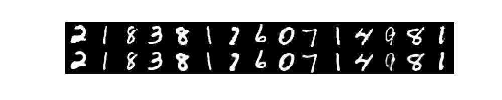
% Version 1.000
% 作用:相当于论文图1中的“Unrolling”部分
% Code provided by Ruslan Salakhutdinov and Geoff Hinton
%
% Permission is granted for anyone to copy, use, modify, or distribute this
% program and accompanying programs and documents for any purpose, provided
% this copyright notice is retained and prominently displayed, along with
% a note saying that the original programs are available from our
% web page.
% The programs and documents are distributed without any warranty, express or
% implied.  As the programs were written for research purposes only, they have
% not been tested to the degree that would be advisable in any important
% application.  All use of these programs is entirely at the user‘s own risk.

% This program fine-tunes an autoencoder with backpropagation.
% Weights of the autoencoder are going to be saved in mnist_weights.mat
% and trainig and test reconstruction errors in mnist_error.mat
% You can also set maxepoch, default value is 200 as in our paper.

maxepoch=200;
fprintf(1,‘\nFine-tuning deep autoencoder by minimizing cross entropy error. \n‘);
fprintf(1,‘60 batches of 1000 cases each. \n‘);

load mnistvh
load mnisthp
load mnisthp2
load mnistpo

makebatches;
[numcases numdims numbatches]=size(batchdata);
N=numcases;

%%%% PREINITIALIZE WEIGHTS OF THE AUTOENCODER %%%%%%%%%%%%%%%%%%%%%%%%%%%%%%%%%%%%%%%%%%%%%
w1=[vishid; hidrecbiases];% [W1;b1] 分别装载每层的权值和偏置值,将它们作为一个整体
w2=[hidpen; penrecbiases];% [W2;b2]
w3=[hidpen2; penrecbiases2];% [W3;b3]
w4=[hidtop; toprecbiases];% [W4;b4]
w5=[hidtop‘; topgenbiases]; % [W4‘;v4]
w6=[hidpen2‘; hidgenbiases2]; % [W3‘;v3]
w7=[hidpen‘; hidgenbiases]; % [W2‘;v2]
w8=[vishid‘; visbiases];% [W1‘;v1]

%%%%%%%%%% END OF PREINITIALIZATIO OF WEIGHTS  %%%%%%%%%%%%%%%%%%%%%%%%%%%%%%%%%%%%%%%%%%%%%

l1=size(w1,1)-1;%每个网络层中节点的个数
l2=size(w2,1)-1;
l3=size(w3,1)-1;
l4=size(w4,1)-1;
l5=size(w5,1)-1;
l6=size(w6,1)-1;
l7=size(w7,1)-1;
l8=size(w8,1)-1;
l9=l1; %输出层节点和输入层的一样
test_err=[];
train_err=[];


for epoch = 1:maxepoch

%%%%%%%%%%%%%%%%%%%% COMPUTE TRAINING RECONSTRUCTION ERROR %%%%%%%%%%%%%%%%%%%%%%%%%%%%%%%%%
err=0;
[numcases numdims numbatches]=size(batchdata);
N=numcases;
 for batch = 1:numbatches
  data = [batchdata(:,:,batch)];
  data = [data ones(N,1)];
  w1probs = 1./(1 + exp(-data*w1)); w1probs = [w1probs  ones(N,1)];%正向传播,计算每一层的输出,且同时在输出上增加一维(值为常量1)
  w2probs = 1./(1 + exp(-w1probs*w2)); w2probs = [w2probs ones(N,1)];
  w3probs = 1./(1 + exp(-w2probs*w3)); w3probs = [w3probs  ones(N,1)];
  w4probs = w3probs*w4; w4probs = [w4probs  ones(N,1)];
  w5probs = 1./(1 + exp(-w4probs*w5)); w5probs = [w5probs  ones(N,1)];
  w6probs = 1./(1 + exp(-w5probs*w6)); w6probs = [w6probs  ones(N,1)];
  w7probs = 1./(1 + exp(-w6probs*w7)); w7probs = [w7probs  ones(N,1)];
  dataout = 1./(1 + exp(-w7probs*w8));
  err= err +  1/N*sum(sum( (data(:,1:end-1)-dataout).^2 )); % 每个batch内的均方误差
  end
 train_err(epoch)=err/numbatches;% 迭代第epoch次的所有样本内的均方误差

%%%%%%%%%%%%%% END OF COMPUTING TRAINING RECONSTRUCTION ERROR %%%%%%%%%%%%%%%%%%%%%%%%%%%%%

%%%% DISPLAY FIGURE TOP ROW REAL DATA BOTTOM ROW RECONSTRUCTIONS %%%%%%%%%%%%%%%%%%%%%%%%%
fprintf(1,‘Displaying in figure 1: Top row - real data, Bottom row -- reconstructions \n‘);
output=[];
 for ii=1:15
  output = [output data(ii,1:end-1)‘ dataout(ii,:)‘];%output为15(因为是显示15个数字)组,每组2列,分别为理论值和重构值
 end
   if epoch==1
   close all
   figure(‘Position‘,[100,600,1000,200]);
   else
   figure(1)
   end
   mnistdisp(output);%显示图片
   drawnow;%刷新屏幕

%%%%%%%%%%%%%%%%%%%% COMPUTE TEST RECONSTRUCTION ERROR %%%%%%%%%%%%%%%%%%%%%%%%%%%%%%%%%%%%
[testnumcases testnumdims testnumbatches]=size(testbatchdata);
N=testnumcases;
err=0;
for batch = 1:testnumbatches
  data = [testbatchdata(:,:,batch)];
  data = [data ones(N,1)];
  w1probs = 1./(1 + exp(-data*w1)); w1probs = [w1probs  ones(N,1)];
  w2probs = 1./(1 + exp(-w1probs*w2)); w2probs = [w2probs ones(N,1)];
  w3probs = 1./(1 + exp(-w2probs*w3)); w3probs = [w3probs  ones(N,1)];
  w4probs = w3probs*w4; w4probs = [w4probs  ones(N,1)];
  w5probs = 1./(1 + exp(-w4probs*w5)); w5probs = [w5probs  ones(N,1)];
  w6probs = 1./(1 + exp(-w5probs*w6)); w6probs = [w6probs  ones(N,1)];
  w7probs = 1./(1 + exp(-w6probs*w7)); w7probs = [w7probs  ones(N,1)];
  dataout = 1./(1 + exp(-w7probs*w8));
  err = err +  1/N*sum(sum( (data(:,1:end-1)-dataout).^2 ));
  end
 test_err(epoch)=err/testnumbatches;
 fprintf(1,‘Before epoch %d Train squared error: %6.3f Test squared error: %6.3f \t \t \n‘,epoch,train_err(epoch),test_err(epoch));

%%%%%%%%%%%%%% END OF COMPUTING TEST RECONSTRUCTION ERROR %%%%%%%%%%%%%%%%%%%%%%%%%%%%%%%%%%

 tt=0;
 for batch = 1:numbatches/10          % 测试样本numbatches是100
 fprintf(1,‘epoch %d batch %d\r‘,epoch,batch);

%%%%%%%%%%% COMBINE 10 MINIBATCHES INTO 1 LARGER MINIBATCH %%%%%%%%%%%%%%%%%%%%%%%%%%%%%%%%%
 tt=tt+1;
 data=[];
 for kk=1:10
  data=[data
        batchdata(:,:,(tt-1)*10+kk)];
 end

%%%%%%%%%%%%%%% PERFORM CONJUGATE GRADIENT WITH 3 LINESEARCHES 共轭梯度线性搜索%%%%%%%%%%%%%%%%%%%%%%%%%%%%%
  max_iter=3;
  VV = [w1(:)‘ w2(:)‘ w3(:)‘ w4(:)‘ w5(:)‘ w6(:)‘ w7(:)‘ w8(:)‘]‘;% 把所有权值(已经包括了偏置值)变成一个大的列向量
  Dim = [l1; l2; l3; l4; l5; l6; l7; l8; l9];%每层网络对应节点的个数(不包括偏置值)

  [X, fX] = minimize(VV,‘CG_MNIST‘,max_iter,Dim,data);

  w1 = reshape(X(1:(l1+1)*l2),l1+1,l2);
  xxx = (l1+1)*l2;
  w2 = reshape(X(xxx+1:xxx+(l2+1)*l3),l2+1,l3);
  xxx = xxx+(l2+1)*l3;
  w3 = reshape(X(xxx+1:xxx+(l3+1)*l4),l3+1,l4);
  xxx = xxx+(l3+1)*l4;
  w4 = reshape(X(xxx+1:xxx+(l4+1)*l5),l4+1,l5);
  xxx = xxx+(l4+1)*l5;
  w5 = reshape(X(xxx+1:xxx+(l5+1)*l6),l5+1,l6);
  xxx = xxx+(l5+1)*l6;
  w6 = reshape(X(xxx+1:xxx+(l6+1)*l7),l6+1,l7);
  xxx = xxx+(l6+1)*l7;
  w7 = reshape(X(xxx+1:xxx+(l7+1)*l8),l7+1,l8);
  xxx = xxx+(l7+1)*l8;
  w8 = reshape(X(xxx+1:xxx+(l8+1)*l9),l8+1,l9);%依次重新赋值为优化后的参数

%%%%%%%%%%%%%%% END OF CONJUGATE GRADIENT WITH 3 LINESEARCHES %%%%%%%%%%%%%%%%%%%%%%%%%%%%%

 end

 save mnist_weights w1 w2 w3 w4 w5 w6 w7 w8
 save mnist_error test_err train_err;

end
CG_MNIST.m
% Version 1.000
% 得到代价函数及其对各权值的偏导数
% Code provided by Ruslan Salakhutdinov and Geoff Hinton
%
% Permission is granted for anyone to copy, use, modify, or distribute this
% program and accompanying programs and documents for any purpose, provided
% this copyright notice is retained and prominently displayed, along with
% a note saying that the original programs are available from our
% web page.
% The programs and documents are distributed without any warranty, express or
% implied.  As the programs were written for research purposes only, they have
% not been tested to the degree that would be advisable in any important
% application.  All use of these programs is entirely at the user‘s own risk.

function [f, df] = CG_MNIST(VV,Dim,XX)
% VV:权值(已经包括了偏置值),为一个大的列向量
% Dim:每层网络对应节点的个数
% XX:训练样本
% f  :代价函数
% df :代价函数对各权值的偏导数


l1 = Dim(1);%每层网络对应节点的个数(不包括偏置值)
l2 = Dim(2);
l3 = Dim(3);
l4= Dim(4);
l5= Dim(5);
l6= Dim(6);
l7= Dim(7);
l8= Dim(8);
l9= Dim(9);
N = size(XX,1);% 样本的个数

% Do decomversion.下面一系列步骤完成权值的矩阵化
 w1 = reshape(VV(1:(l1+1)*l2),l1+1,l2);% VV是一个长的列向量,它包括偏置值和权值,这里取出的向量已经包括了偏置值
 xxx = (l1+1)*l2; %xxx 表示已经使用了的长度
 w2 = reshape(VV(xxx+1:xxx+(l2+1)*l3),l2+1,l3);
 xxx = xxx+(l2+1)*l3;
 w3 = reshape(VV(xxx+1:xxx+(l3+1)*l4),l3+1,l4);
 xxx = xxx+(l3+1)*l4;
 w4 = reshape(VV(xxx+1:xxx+(l4+1)*l5),l4+1,l5);
 xxx = xxx+(l4+1)*l5;
 w5 = reshape(VV(xxx+1:xxx+(l5+1)*l6),l5+1,l6);
 xxx = xxx+(l5+1)*l6;
 w6 = reshape(VV(xxx+1:xxx+(l6+1)*l7),l6+1,l7);
 xxx = xxx+(l6+1)*l7;
 w7 = reshape(VV(xxx+1:xxx+(l7+1)*l8),l7+1,l8);
 xxx = xxx+(l7+1)*l8;
 w8 = reshape(VV(xxx+1:xxx+(l8+1)*l9),l8+1,l9);


  XX = [XX ones(N,1)];
  w1probs = 1./(1 + exp(-XX*w1)); w1probs = [w1probs  ones(N,1)];
  w2probs = 1./(1 + exp(-w1probs*w2)); w2probs = [w2probs ones(N,1)];
  w3probs = 1./(1 + exp(-w2probs*w3)); w3probs = [w3probs  ones(N,1)];
  w4probs = w3probs*w4; w4probs = [w4probs  ones(N,1)];
  w5probs = 1./(1 + exp(-w4probs*w5)); w5probs = [w5probs  ones(N,1)];
  w6probs = 1./(1 + exp(-w5probs*w6)); w6probs = [w6probs  ones(N,1)];
  w7probs = 1./(1 + exp(-w6probs*w7)); w7probs = [w7probs  ones(N,1)];
  XXout = 1./(1 + exp(-w7probs*w8));

f = -1/N*sum(sum( XX(:,1:end-1).*log(XXout) + (1-XX(:,1:end-1)).*log(1-XXout)));%原始数据和重构数据的代价函数,怎么推导的?
IO = 1/N*(XXout-XX(:,1:end-1));% 误差
Ix8=IO;
dw8 =  w7probs‘*Ix8;%输出层的误差项,但是这个公式怎么和以前介绍的不同,因为它的误差评价标准是交叉熵,不是MSE

Ix7 = (Ix8*w8‘).*w7probs.*(1-w7probs);
Ix7 = Ix7(:,1:end-1);
dw7 =  w6probs‘*Ix7;

Ix6 = (Ix7*w7‘).*w6probs.*(1-w6probs);
Ix6 = Ix6(:,1:end-1);
dw6 =  w5probs‘*Ix6;

Ix5 = (Ix6*w6‘).*w5probs.*(1-w5probs);
Ix5 = Ix5(:,1:end-1);
dw5 =  w4probs‘*Ix5;

Ix4 = (Ix5*w5‘);
Ix4 = Ix4(:,1:end-1);
dw4 =  w3probs‘*Ix4;

Ix3 = (Ix4*w4‘).*w3probs.*(1-w3probs);
Ix3 = Ix3(:,1:end-1);
dw3 =  w2probs‘*Ix3;

Ix2 = (Ix3*w3‘).*w2probs.*(1-w2probs);
Ix2 = Ix2(:,1:end-1);
dw2 =  w1probs‘*Ix2;

Ix1 = (Ix2*w2‘).*w1probs.*(1-w1probs);
Ix1 = Ix1(:,1:end-1);
dw1 =  XX‘*Ix1;

df = [dw1(:)‘ dw2(:)‘ dw3(:)‘ dw4(:)‘ dw5(:)‘ dw6(:)‘  dw7(:)‘  dw8(:)‘  ]‘; %网络代价函数的偏导数
minimize.m
function [X, fX, i] = minimize(X, f, length, varargin)
%作用:利用共轭梯度下降法对目标函数进行优化
% Minimize a differentiable multivariate function.
%
% Usage: [X, fX, i] = minimize(X, f, length, P1, P2, P3, ... )
%
% where the starting point is given by "X" (D by 1), and the function named in
% the string "f", must return a function value and a vector of partial
% derivatives of f wrt X, the "length" gives the length of the run: if it is
% positive, it gives the maximum number of line searches, if negative its
% absolute gives the maximum allowed number of function evaluations. You can
% (optionally) give "length" a second component, which will indicate the
% reduction in function value to be expected in the first line-search (defaults
% to 1.0). The parameters P1, P2, P3, ... are passed on to the function f.
%
% The function returns when either its length is up, or if no further progress
% can be made (ie, we are at a (local) minimum, or so close that due to
% numerical problems, we cannot get any closer). NOTE: If the function
% terminates within a few iterations, it could be an indication that the
% function values and derivatives are not consistent (ie, there may be a bug in
% the implementation of your "f" function). The function returns the found
% solution "X", a vector of function values "fX" indicating the progress made
% and "i" the number of iterations (line searches or function evaluations,
% depending on the sign of "length") used.
%
% The Polack-Ribiere flavour of conjugate gradients is used to compute search
% directions, and a line search using quadratic and cubic polynomial
% approximations and the Wolfe-Powell stopping criteria is used together with
% the slope ratio method for guessing initial step sizes. Additionally a bunch
% of checks are made to make sure that exploration is taking place and that
% extrapolation will not be unboundedly large.
%
% See also: checkgrad
%
% Copyright (C) 2001 - 2006 by Carl Edward Rasmussen (2006-09-08).

INT = 0.1;    % don‘t reevaluate within 0.1 of the limit of the current bracket
EXT = 3.0;                  % extrapolate maximum 3 times the current step-size
MAX = 20;                         % max 20 function evaluations per line search
RATIO = 10;                                       % maximum allowed slope ratio
SIG = 0.1; RHO = SIG/2; % SIG and RHO are the constants controlling the Wolfe-
% Powell conditions. SIG is the maximum allowed absolute ratio between
% previous and new slopes (derivatives in the search direction), thus setting
% SIG to low (positive) values forces higher precision in the line-searches.
% RHO is the minimum allowed fraction of the expected (from the slope at the
% initial point in the linesearch). Constants must satisfy 0 < RHO < SIG < 1.
% Tuning of SIG (depending on the nature of the function to be optimized) may
% speed up the minimization; it is probably not worth playing much with RHO.

% The code falls naturally into 3 parts, after the initial line search is
% started in the direction of steepest descent. 1) we first enter a while loop
% which uses point 1 (p1) and (p2) to compute an extrapolation (p3), until we
% have extrapolated far enough (Wolfe-Powell conditions). 2) if necessary, we
% enter the second loop which takes p2, p3 and p4 chooses the subinterval
% containing a (local) minimum, and interpolates it, unil an acceptable point
% is found (Wolfe-Powell conditions). Note, that points are always maintained
% in order p0 <= p1 <= p2 < p3 < p4. 3) compute a new search direction using
% conjugate gradients (Polack-Ribiere flavour), or revert to steepest if there
% was a problem in the previous line-search. Return the best value so far, if
% two consecutive line-searches fail, or whenever we run out of function
% evaluations or line-searches. During extrapolation, the "f" function may fail
% either with an error or returning Nan or Inf, and minimize should handle this
% gracefully.

if max(size(length)) == 2, red=length(2); length=length(1); else red=1; end
if length>0, S=‘Linesearch‘; else S=‘Function evaluation‘; end

i = 0;                                            % zero the run length counter
ls_failed = 0;                             % no previous line search has failed
[f0 df0] = feval(f, X, varargin{:});          % get function value and gradient
fX = f0;
i = i + (length<0);                                            % count epochs?!
s = -df0; d0 = -s‘*s;           % initial search direction (steepest) and slope
x3 = red/(1-d0);                                  % initial step is red/(|s|+1)

while i < abs(length)                                      % while not finished
  i = i + (length>0);                                      % count iterations?!

  X0 = X; F0 = f0; dF0 = df0;                   % make a copy of current values
  if length>0, M = MAX; else M = min(MAX, -length-i); end

  while 1                             % keep extrapolating as long as necessary
    x2 = 0; f2 = f0; d2 = d0; f3 = f0; df3 = df0;
    success = 0;
    while ~success && M > 0
      try
        M = M - 1; i = i + (length<0);                         % count epochs?!
        [f3 df3] = feval(f, X+x3*s, varargin{:});
        if isnan(f3) || isinf(f3) || any(isnan(df3)+isinf(df3)), error(‘‘), end
        success = 1;
      catch                                % catch any error which occured in f
        x3 = (x2+x3)/2;                                  % bisect and try again
      end
    end
    if f3 < F0, X0 = X+x3*s; F0 = f3; dF0 = df3; end         % keep best values
    d3 = df3‘*s;                                                    % new slope
    if d3 > SIG*d0 || f3 > f0+x3*RHO*d0 || M == 0  % are we done extrapolating?
      break
    end
    x1 = x2; f1 = f2; d1 = d2;                        % move point 2 to point 1
    x2 = x3; f2 = f3; d2 = d3;                        % move point 3 to point 2
    A = 6*(f1-f2)+3*(d2+d1)*(x2-x1);                 % make cubic extrapolation
    B = 3*(f2-f1)-(2*d1+d2)*(x2-x1);
    x3 = x1-d1*(x2-x1)^2/(B+sqrt(B*B-A*d1*(x2-x1))); % num. error possible, ok!
    if ~isreal(x3) || isnan(x3) || isinf(x3) || x3 < 0 % num prob | wrong sign?
      x3 = x2*EXT;                                 % extrapolate maximum amount
    elseif x3 > x2*EXT                  % new point beyond extrapolation limit?
      x3 = x2*EXT;                                 % extrapolate maximum amount
    elseif x3 < x2+INT*(x2-x1)         % new point too close to previous point?
      x3 = x2+INT*(x2-x1);
    end
  end                                                       % end extrapolation

  while (abs(d3) > -SIG*d0 || f3 > f0+x3*RHO*d0) && M > 0  % keep interpolating
    if d3 > 0 || f3 > f0+x3*RHO*d0                         % choose subinterval
      x4 = x3; f4 = f3; d4 = d3;                      % move point 3 to point 4
    else
      x2 = x3; f2 = f3; d2 = d3;                      % move point 3 to point 2
    end
    if f4 > f0
      x3 = x2-(0.5*d2*(x4-x2)^2)/(f4-f2-d2*(x4-x2));  % quadratic interpolation
    else
      A = 6*(f2-f4)/(x4-x2)+3*(d4+d2);                    % cubic interpolation
      B = 3*(f4-f2)-(2*d2+d4)*(x4-x2);
      x3 = x2+(sqrt(B*B-A*d2*(x4-x2)^2)-B)/A;        % num. error possible, ok!
    end
    if isnan(x3) || isinf(x3)
      x3 = (x2+x4)/2;               % if we had a numerical problem then bisect
    end
    x3 = max(min(x3, x4-INT*(x4-x2)),x2+INT*(x4-x2));  % don‘t accept too close
    [f3 df3] = feval(f, X+x3*s, varargin{:});
    if f3 < F0, X0 = X+x3*s; F0 = f3; dF0 = df3; end         % keep best values
    M = M - 1; i = i + (length<0);                             % count epochs?!
    d3 = df3‘*s;                                                    % new slope
  end                                                       % end interpolation

  if abs(d3) < -SIG*d0 && f3 < f0+x3*RHO*d0          % if line search succeeded
    X = X+x3*s; f0 = f3; fX = [fX‘ f0]‘;                     % update variables
    fprintf(‘%s %6i;  Value %4.6e\r‘, S, i, f0);
    s = (df3‘*df3-df0‘*df3)/(df0‘*df0)*s - df3;   % Polack-Ribiere CG direction
    df0 = df3;                                               % swap derivatives
    d3 = d0; d0 = df0‘*s;
    if d0 > 0                                      % new slope must be negative
      s = -df0; d0 = -s‘*s;                  % otherwise use steepest direction
    end
    x3 = x3 * min(RATIO, d3/(d0-realmin));          % slope ratio but max RATIO
    ls_failed = 0;                              % this line search did not fail
  else
    X = X0; f0 = F0; df0 = dF0;                     % restore best point so far
    if ls_failed || i > abs(length)         % line search failed twice in a row
      break;                             % or we ran out of time, so we give up
    end
    s = -df0; d0 = -s‘*s;                                        % try steepest
    x3 = 1/(1-d0);
    ls_failed = 1;                                    % this line search failed
  end
end
fprintf(‘\n‘);
参考文献
Deep Learning 16:用自编码器对数据进行降维_读论文“Reducing the Dimensionality of Data with Neural Networks”的笔记
原文:http://www.cnblogs.com/dmzhuo/p/5072808.html