代码:
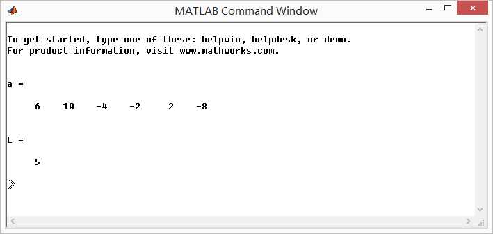
h = [-4, 1, -1, -2, 5, 6, 5, -2, -1, 1, -4];
M = length(h); n = 0:M-1;
[Hr, w, a, L] = Hr_Type1(h);
a
L

amax = max(a) + 1; amin = min(a) - 1;

figure(‘NumberTitle‘, ‘off‘, ‘Name‘, ‘Exameple 7.4‘)
set(gcf,‘Color‘,‘white‘);

subplot(2,2,1); stem(n, h); axis([-1, 2*L+1, amin, amax]);
xlabel(‘n‘); ylabel(‘h(n)‘); title(‘Impulse Response‘); grid on;

subplot(2,2,3); stem(0:L, a); axis([-1, 2*L+1, amin, amax]);
xlabel(‘n‘); ylabel(‘a(n)‘); title(‘a(n) coefficients‘); grid on;

subplot(2,2,2); plot(w/pi, Hr); grid on;
xlabel(‘frequency in \pi units‘); ylabel(‘Hr‘); title(‘Type-1 Amplitude Response‘);

subplot(2,2,4); zplane(h); grid on;
xlabel(‘real axis‘); ylabel(‘imaginary axis‘); title(‘Pole-Zero Plot‘);
运行结果:
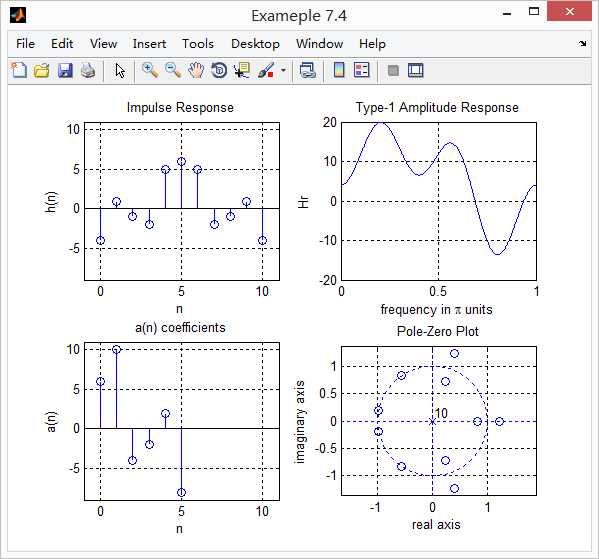
从上述图中看出,在ω=0,或者ω=π,振幅谱Hr(ω)没有任何限制。
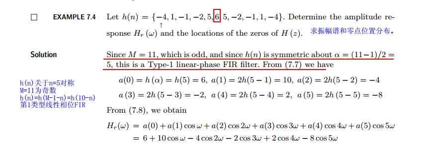
《DSP using MATLAB》示例Example7.4
原文:http://www.cnblogs.com/ky027wh-sx/p/6618977.html