 ?
?
#!/usr/bin/env python
# -*- coding: utf-8 -*-
# Created by xuehz on 2017/4/9
import numpy as np
import matplotlib as mpl
import matplotlib.pyplot as plt
from scipy.stats import norm, poisson
import time
from scipy.optimize import leastsq
from scipy import stats
import scipy.optimize as opt
import matplotlib.pyplot as plt
from scipy.stats import norm, poisson
from scipy.interpolate import BarycentricInterpolator
from scipy.interpolate import CubicSpline
from scipy import stats
import math
mpl.rcParams['font.sans-serif'] = [u'SimHei'] #FangSong/黑体 FangSong/KaiTi
mpl.rcParams['axes.unicode_minus'] = False
def f(x):
y = np.ones_like(x)
i = x > 0
y[i] = np.power(x[i], x[i])
i = x < 0
y[i] = np.power(-x[i], -x[i])
return y
def residual(t, x, y):
return y - (t[0] * x ** 2 + t[1] * x + t[2])
def residual2(t, x, y):
print t[0], t[1]
return y - (t[0]*np.sin(t[1]*x) + t[2])
if __name__ == '__main__':
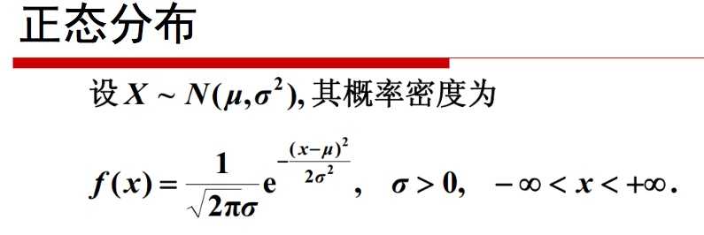
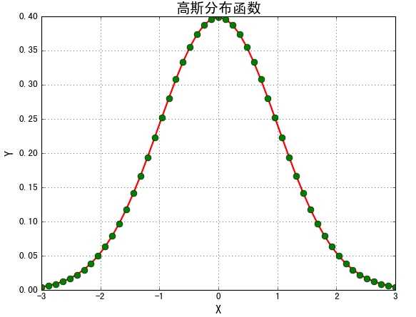
#绘制正态分布概率密度函数
# mu = 0
# sigma = 1
# x = np.linspace(mu - 3 * sigma, mu + 3 * sigma, 51)
# y = np.exp(-(x - mu) ** 2 / (2 * sigma ** 2)) / (math.sqrt(2 * math.pi) * sigma)
# print x.shape
# print 'x = \n', x
# print y.shape
# print 'y = \n', y
# #plt.plot(x, y, 'ro-', linewidth=2)
# plt.figure(facecolor='w')
# plt.plot(x, y, 'r-', x, y, 'go', linewidth=2, markersize=8)
# plt.xlabel('X', fontsize=15)
# plt.ylabel('Y', fontsize=15)
# plt.title(u'高斯分布函数', fontsize=18)
# plt.grid(True)
# plt.show()
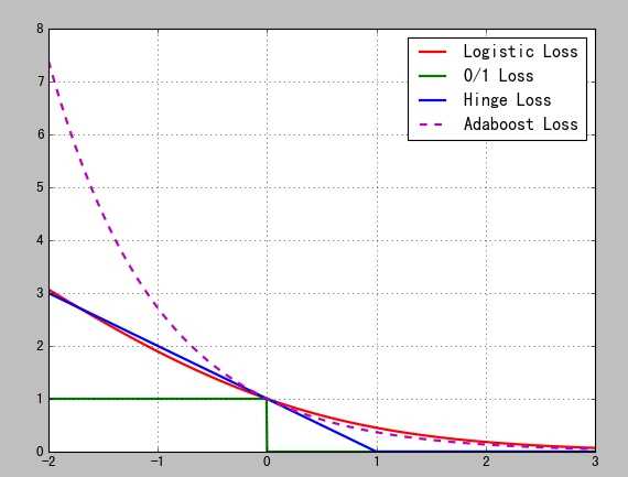
#损失函数:Logistic损失(-1,1)/SVM Hinge损失/ 0/1损失
# x = np.array(np.linspace(start=-2, stop=3, num=1001, dtype=np.float))
# y_logit = np.log(1 + np.exp(-x)) / math.log(2)
# y_boost = np.exp(-x)
# y_01 = x < 0
# y_hinge = 1.0 - x
# y_hinge[y_hinge < 0] = 0
# plt.plot(x, y_logit, 'r-', label='Logistic Loss', linewidth=2)
# plt.plot(x, y_01, 'g-', label='0/1 Loss', linewidth=2)
# plt.plot(x, y_hinge, 'b-', label='Hinge Loss', linewidth=2)
# plt.plot(x, y_boost, 'm--', label='Adaboost Loss', linewidth=2)
# plt.grid()
# plt.legend(loc='upper right')
# # plt.savefig('1.png')
# plt.show()
#x^x
# x = np.linspace(-1.3, 1.3, 101)
# y = f(x)
# plt.plot(x, y, 'g-', label='x^x', linewidth=2)
# plt.grid()
# plt.legend(loc='upper left')
# plt.show()
# # 胸型线
# x = np.arange(1, 0, -0.001)
# y = (-3 * x * np.log(x) + np.exp(-(40 * (x - 1 / np.e)) ** 4) / 25) / 2
# plt.figure(figsize=(5,7), facecolor='w')
# plt.plot(y, x, 'r-', linewidth=2)
# plt.grid(True)
# plt.title(u'胸型线', fontsize=20)
# # plt.savefig('breast.png')
# plt.show()
#
#
# # 心形线
# t = np.linspace(0, 2*np.pi, 100)
# x = 16 * np.sin(t) ** 3
# y = 13 * np.cos(t) - 5 * np.cos(2*t) - 2 * np.cos(3*t) - np.cos(4*t)
# plt.plot(x, y, 'r-', linewidth=2)
# plt.grid(True)
# plt.show()
#
# # 渐开线
# t = np.linspace(0, 50, num=1000)
# x = t*np.sin(t) + np.cos(t)
# y = np.sin(t) - t*np.cos(t)
# plt.plot(x, y, 'r-', linewidth=2)
# plt.grid()
# plt.show()
#
# # Bar
# x = np.arange(0, 10, 0.1)
# y = np.sin(x)
# plt.bar(x, y, width=0.04, linewidth=0.2)
# plt.plot(x, y, 'r--', linewidth=2)
# plt.title(u'Sin曲线')
# plt.xticks(rotation=-60)
# plt.xlabel('X')
# plt.ylabel('Y')
# plt.grid()
# plt.show()
# # # 6. 概率分布
# # 6.1 均匀分布
# x = np.random.rand(10000)
# t = np.arange(len(x))
# #plt.hist(x, 30, color='m', alpha=0.5, label=u'均匀分布')
# plt.plot(t, x, 'r-', label=u'均匀分布')
# plt.legend(loc='upper left')
# plt.grid()
# plt.show()
# # 6.2 验证中心极限定理
# t = 1000
# a = np.zeros(10000)
# for i in range(t):
# a += np.random.uniform(-5, 5, 10000)
# a /= t
# plt.hist(a, bins=30, color='g', alpha=0.5, normed=True, label=u'均匀分布叠加')
# plt.legend(loc='upper left')
# plt.grid()
# plt.show()
#
# #6.21 其他分布的中心极限定理
# lamda = 10
# p = stats.poisson(lamda)
# y = p.rvs(size=1000)
# mx = 30
# r = (0, mx)
# bins = r[1] - r[0]
# plt.figure(figsize=(10, 8), facecolor='w')
# plt.subplot(121)
# plt.hist(y, bins=bins, range=r, color='g', alpha=0.8, normed=True)
# t = np.arange(0, mx+1)
# plt.plot(t, p.pmf(t), 'ro-', lw=2)
# plt.grid(True)
# N = 1000
# M = 10000
# plt.subplot(122)
# a = np.zeros(M, dtype=np.float)
# p = stats.poisson(lamda)
# for i in np.arange(N):
# y = p.rvs(size=M)
# a += y
# a /= N
# plt.hist(a, bins=20, color='g', alpha=0.8, normed=True)
# plt.grid(b=True)
# plt.show()
# # 6.3 Poisson分布
# x = np.random.poisson(lam=5, size=10000)
# print x
# pillar = 15
# a = plt.hist(x, bins=pillar, normed=True, range=[0, pillar], color='g', alpha=0.5)
# plt.grid()
# plt.show()
# print a
# print a[0].sum()
#
# # 6.4 直方图的使用
# mu = 2
# sigma = 3
# data = mu + sigma * np.random.randn(1000)
# h = plt.hist(data, 30, normed=1, color='#a0a0ff')
# x = h[1]
# y = norm.pdf(x, loc=mu, scale=sigma)
# plt.plot(x, y, 'r--', x, y, 'ro', linewidth=2, markersize=4)
# plt.grid()
# plt.show()
# # 6.5 插值
# rv = poisson(5)
# x1 = a[1]
# y1 = rv.pmf(x1)
# itp = BarycentricInterpolator(x1, y1) # 重心插值
# x2 = np.linspace(x.min(), x.max(), 50)
# y2 = itp(x2)
# cs = scipy.interpolate.CubicSpline(x1, y1) # 三次样条插值
# plt.plot(x2, cs(x2), 'm--', linewidth=5, label='CubicSpine') # 三次样条插值
# plt.plot(x2, y2, 'g-', linewidth=3, label='BarycentricInterpolator') # 重心插值
# plt.plot(x1, y1, 'r-', linewidth=1, label='Actural Value') # 原始值
# plt.legend(loc='upper right')
# plt.grid()
# plt.show()
# 8.1 scipy
#线性回归例1
x = np.linspace(-2, 2, 50)
A, B, C = 2, 3, -1
y = (A * x ** 2 + B * x + C) + np.random.rand(len(x))*0.75
t = leastsq(residual, [0, 0, 0], args=(x, y))
theta = t[0]
print '真实值:', A, B, C
print '预测值:', theta
y_hat = theta[0] * x ** 2 + theta[1] * x + theta[2]
plt.plot(x, y, 'r-', linewidth=2, label=u'Actual')
plt.plot(x, y_hat, 'g-', linewidth=2, label=u'Predict')
plt.legend(loc='upper left')
plt.grid()
plt.show()
# 线性回归例2
x = np.linspace(0, 5, 100)
a = 5
w = 1.5
phi = -2
y = a * np.sin(w*x) + phi + np.random.rand(len(x))*0.5
t = leastsq(residual2, [3, 5, 1], args=(x, y))
theta = t[0]
print '真实值:', a, w, phi
print '预测值:', theta
y_hat = theta[0] * np.sin(theta[1] * x) + theta[2]
plt.plot(x, y, 'r-', linewidth=2, label='Actual')
plt.plot(x, y_hat, 'g-', linewidth=2, label='Predict')
plt.legend(loc='lower left')
plt.grid()
plt.show()
# marker description
# ”.” point
# ”,” pixel
# “o” circle
# “v” triangle_down
# “^” triangle_up
# “<” triangle_left
# “>” triangle_right
# “1” tri_down
# “2” tri_up
# “3” tri_left
# “4” tri_right
# “8” octagon
# “s” square
# “p” pentagon
# “*” star
# “h” hexagon1
# “H” hexagon2
# “+” plus
# “x” x
# “D” diamond
# “d” thin_diamond
# “|” vline
# “_” hline
# TICKLEFT tickleft
# TICKRIGHT tickright
# TICKUP tickup
# TICKDOWN tickdown
# CARETLEFT caretleft
# CARETRIGHT caretright
# CARETUP caretup
# CARETDOWN caretdown
 ?
?
 ?
?
原文:http://www.cnblogs.com/xuehaozhe/p/python-ji-chu2-hua-tu.html