代码:
%% ------------------------------------------------------------------------
%%            Output Info about this m-file
fprintf(‘\n***********************************************************\n‘);
fprintf(‘        <DSP using MATLAB> Exameple 9.12 \n\n‘);

time_stamp = datestr(now, 31);
[wkd1, wkd2] = weekday(today, ‘long‘);
fprintf(‘      Now is %20s, and it is %7s  \n\n‘, time_stamp, wkd2);
%% ------------------------------------------------------------------------

% Given Parameters:

D = 2; Rp = 0.1; As = 30; wp = pi/D; ws = wp+0.1*pi;

% Filter Design:
[delta1, delta2] = db2delta(Rp, As);

[N, F, A, weights] = firpmord([wp, ws]/pi, [1, 0], [delta1, delta2], 2);
h = firpm(N, F, A, weights);
delay = N/2;                        % delay imparted by the filter


%% -----------------------------------------------------------------
%%                             Plot
%% -----------------------------------------------------------------

% Input signal x1(n) = cos(2*pi*n/16)
n = [0:256]; x = cos(pi*n/8);
n1 = n(1:33); x1 = x(33:65);            % for plotting purposes

Hf1 = figure(‘units‘, ‘inches‘, ‘position‘, [1, 1, 8, 6], ...
	‘paperunits‘, ‘inches‘, ‘paperposition‘, [0, 0, 6, 4], ...
	‘NumberTitle‘, ‘off‘, ‘Name‘, ‘Exameple 9.12‘);
set(gcf,‘Color‘,‘white‘);

TF = 10;

subplot(2, 2, 1);
Hs1 = stem(n1, x1, ‘filled‘); set(Hs1, ‘markersize‘, 2, ‘color‘, ‘g‘);
axis([-2, 34, -1.2, 1.2]); grid on;
xlabel(‘n‘, ‘vertical‘, ‘middle‘); ylabel(‘Amplitude‘);
title(‘Input Singal: x1(n) = cos(\pin/8) ‘, ‘fontsize‘, TF, ‘vertical‘, ‘baseline‘);
set(gca, ‘xtick‘, [0:8:32]);
set(gca, ‘ytick‘, [-1, 0, 1]);

% Decimation of x1(n): D = 2
y = upfirdn(x, h, 1, D);
m = delay+1:1:128/D+delay+1; y = y(m); m = 0:16; y = y(16:32);

subplot(2, 2, 3);
Hs2 = stem(m, y, ‘filled‘); set(Hs2, ‘markersize‘, 2, ‘color‘, ‘m‘);
axis([-1, 17, -1.2, 1.2]); grid on;
xlabel(‘m‘, ‘vertical‘, ‘middle‘); ylabel(‘Amplitude‘, ‘vertical‘, ‘cap‘);
title(‘Output Singal: y1(n): D=2‘, ‘fontsize‘, TF, ‘vertical‘, ‘baseline‘);
set(gca, ‘xtick‘, [0:8:32]/D);
set(gca, ‘ytick‘, [-1, 0, 1]);

% Input signal x2(n) = cos(8*pi*n/16)
n = [0:256]; x = cos(8*pi*n/(16));
n2 = n(1:33); x2 = x(33:65);            % for plotting purposes

subplot(2, 2, 2);
Hs3 = stem(n2, x2, ‘filled‘); set(Hs3, ‘markersize‘, 2, ‘color‘, ‘g‘);
axis([-2, 34, -1.2, 1.2]); grid on;
xlabel(‘n‘, ‘vertical‘, ‘middle‘); ylabel(‘Amplitude‘, ‘vertical‘, ‘cap‘);
title(‘Input Singal: x2(n)=cos(\pin/2) ‘, ‘fontsize‘, TF, ‘vertical‘, ‘baseline‘);
set(gca, ‘xtick‘, [0:8:32]);
set(gca, ‘ytick‘, [-1, 0, 1]);

% Decimation of x2(n): D = 2
y = upfirdn(x, [h], 1, D);           % y = downsample(conv(x,h),2);
m = delay+1:1:128/D+delay+1; y = y(m); m = 0:16; y = y(16:32);

subplot(2, 2, 4);
Hs4 = stem(m, y, ‘filled‘); set(Hs4, ‘markersize‘, 2, ‘color‘, ‘m‘);
axis([-1, 17, -1.2, 1.2]); grid on;
xlabel(‘m‘, ‘vertical‘, ‘middle‘); ylabel(‘Amplitude‘, ‘vertical‘, ‘cap‘);
title(‘Output Singal: y2(n): D=2‘, ‘fontsize‘, TF, ‘vertical‘, ‘baseline‘);
set(gca, ‘xtick‘, [0:8:32]/D);
set(gca, ‘ytick‘, [-1, 0, 1]);
运行结果:
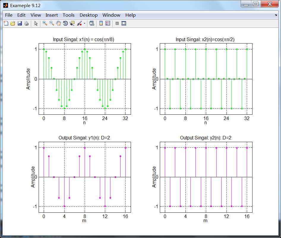
左半边的图展示了x1(n)和相应减采样结果信号y1(n),右半边展示了x2(n)和相应减采样y2(n)。两种情况下减采样
看上去都正确。如果我们选π/2以上的任何频率,那么滤波器将会衰减或消除信号。
《DSP using MATLAB》 示例 Example 9.12
原文:http://www.cnblogs.com/ky027wh-sx/p/6922495.html