给你多组数据集,例如给你很多房子的面积、房子距离市中心的距离、房子的价格,然后再给你一组面积、 距离,让你预测房价。这类问题称为回归问题。
回归问题(Regression) 是给定多个自变量、一个因变量以及代表它们之间关系的一些训练样本,来确定它们的关系。其中最简单的一类是线性回归(Linear Degression)。
线性回归函数的形式如下:
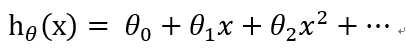 (1)
(1)
θj 是我们要求的系数。接下来介绍一下求θ 的两种方法,梯度下降(Gradient Descent)和正规方程(Normal Rquation )。
1. 梯度下降法
描述:梯度下降法(Gradient descent)是一个一阶最优化算法,通常也称为最速下降法。 要使用梯度下降法找到一个函数的局部极小值,必须向函数上当前点对应梯度(或者是近似梯度)的反方向的规定步长距离点进行迭代搜索。如果相反地向梯度正方向迭代进行搜索,则会接近函数的局部极大值点;这个过程则被称为梯度上升法。
公式:
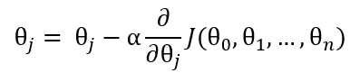 (2)
(2)
其中,J(θ) 称为代价函数(Cost Function )或损失函数(Loss Function), 用来量度预测结果和标准结果之间的误差,常见的有交叉熵,均方误差,平均绝对值误差等。在这里使用均方误差。α是学习速率,取值自定,一般取比较小的数,如0.03
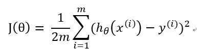 (3)
(3)
( hθ(x) 是x经过待求的函数得出的结果,y(i) 是数据集中的结果)
公式(2)的旨在求出最小的θj,把代价函数J(θ)降到最小。它的原理是θ不停地迭代,减去θ对应的代价函数在x的偏导,如果偏导是正的,那么J(θ)在该方向单增,减去这个正数后θ变小,J(θ)也会跟着变小;反之,如果偏导是负的,J(θ)单减,原θ减负数,θ变大,J(θ)减小。无论怎样,J(θ)都朝着减小的方向变化。值得注意的是,如果学习速率α偏大,那么θ在做差的话可能减过头甚至得到的新J(θ)比原来还要大,而如果学习速率α偏小,那么花费的时间会变长。
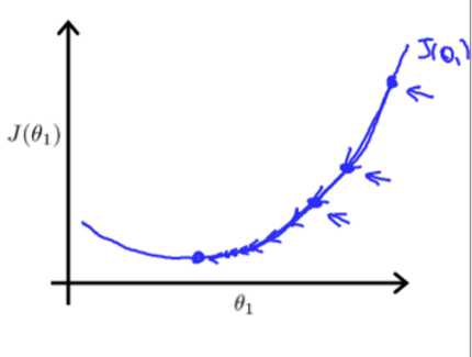 (结合图像更直观)
梯度下降算法是一个不断迭代的过程,需要不断重复公式(2),直到J(θ)符合预期误差或者达到足够的迭代次数。
具体步骤如下:
step0: 初始化α,θ(任意值)和迭代次数;
step1:利用公式(3) ,求J(θ);
step2:利用公式(2),本次迭代的新θ;
step3:重复step1 - step2
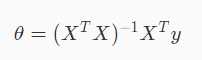
2. 正规方程
利用正规方程可以直接计算计算θ,前提是(XTX)必须可逆
3. matlab实现
3.1 初始化参数
data = load(‘ex1data1.txt‘);
X = data(:, 1); y = data(:, 2);
m = length(y); % number of training examples
plotData(X, y)

X = [ones(m, 1), data(:,1)]; % Add a column of ones to x
theta = zeros(2, 1); % initialize fitting parameters

% Some gradient descent settings
iterations = 1500;
alpha = 0.01;
3.2 计算代价函数
3.3 梯度下降并迭代
function [theta, J_history] = gradientDescent(X, y, theta, alpha, num_iters)
%GRADIENTDESCENT Performs gradient descent to learn theta
%   theta = GRADIENTDESCENT(X, y, theta, alpha, num_iters) updates theta by
%   taking num_iters gradient steps with learning rate alpha

% Initialize some useful values
m = length(y); % number of training examples
J_history = zeros(num_iters, 1);
x = X(:,2);
for iter = 1:num_iters

    % ====================== YOUR CODE HERE ======================
    % Instructions: Perform a single gradient step on the parameter vector
    %               theta.
    %
    % Hint: While debugging, it can be useful to print out the values
    %       of the cost function (computeCost) and gradient here.
    %

    J = alpha * (1/m) * (X * theta - y)‘ ;

    theta(1) = theta(1) - J * ones(m,1);
    theta(2) = theta(2) - J * x;

    % ============================================================

    % Save the cost J in every iteration
    J_history(iter) = computeCost(X, y, theta);

end
end
3.4 绘图
% Grid over which we will calculate J
theta0_vals = linspace(-10, 10, 100);
theta1_vals = linspace(-1, 4, 100);

% initialize J_vals to a matrix of 0‘s
J_vals = zeros(length(theta0_vals), length(theta1_vals));

% Fill out J_vals
for i = 1:length(theta0_vals)
    for j = 1:length(theta1_vals)
      t = [theta0_vals(i); theta1_vals(j)];
      J_vals(i,j) = computeCost(X, y, t);
    end
end


% Because of the way meshgrids work in the surf command, we need to
% transpose J_vals before calling surf, or else the axes will be flipped
J_vals = J_vals‘;
% Surface plot
figure;
surf(theta0_vals, theta1_vals, J_vals)
xlabel(‘\theta_0‘); ylabel(‘\theta_1‘);

% Contour plot
figure;
% Plot J_vals as 15 contours spaced logarithmically between 0.01 and 100
contour(theta0_vals, theta1_vals, J_vals, logspace(-2, 3, 20))
xlabel(‘\theta_0‘); ylabel(‘\theta_1‘);
hold on;
plot(theta(1), theta(2), ‘rx‘, ‘MarkerSize‘, 10, ‘LineWidth‘, 2);
原文:https://www.cnblogs.com/lvdalao/p/9520905.html