主要内容:
一.Mini-Batch Gradient descent
二.Momentum
四.RMSprop
五.Adam
六.优化算法性能比较
一.Mini-Batch Gradient descent
1.一般地,有三种梯度下降算法:
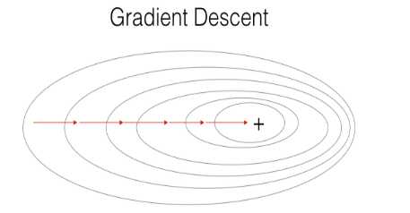
1)(Batch )Gradient Descent,即我们平常所用的。它在每次求梯度的时候用上所有数据集,此种方式适合用在数据集规模不大的情况下。
X = data_input
Y = labels
parameters = initialize_parameters(layers_dims)
for i in range(0, num_iterations):
    # Forward propagation
    a, caches = forward_propagation(X, parameters)
    # Compute cost.
    cost = compute_cost(a, Y)
    # Backward propagation.
    grads = backward_propagation(a, caches, parameters)
    # Update parameters.
    parameters = update_parameters(parameters, grads)
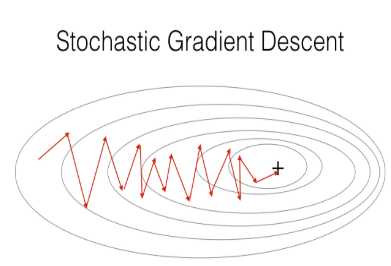
2)Stochastic Gradient Descent,它在每次求梯度的时候只用上一个数据,无疑,这种方式对噪声敏感,且梯度的方向往往偏离较大。
X = data_input
Y = labels
parameters = initialize_parameters(layers_dims)
for i in range(0, num_iterations):
    for j in range(0, m):
        # Forward propagation
        a, caches = forward_propagation(X[:,j], parameters)
        # Compute cost
        cost = compute_cost(a, Y[:,j])
        # Backward propagation
        grads = backward_propagation(a, caches, parameters)
        # Update parameters.
        parameters = update_parameters(parameters, grads)
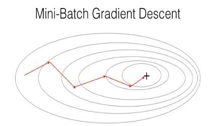
3)Mini-Batch Gradient Descent,就是是在计算梯度时,仅仅利用数据集中的一部分,而不是全部。这样在忽略了梯度准确性的代价下,提升了梯度下降收敛的速度。mini-batch适合用在数据集规模庞大的时。由此可知,min-batch gradient descent 在 batch gradient descent 和 stochastic gradient descent 这两个极端之前采取了折衷的方式,这样既考虑到了梯度的精确性,又考虑到了训练速度,或许这就是中庸之道。
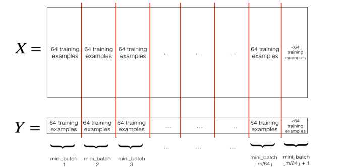
2.执行min-batch gradient descent之前,需要对数据集进行两步操作
1)Shuffle,即打乱数据集的顺序,以此保证数据集随机地分配到mini-batches中。
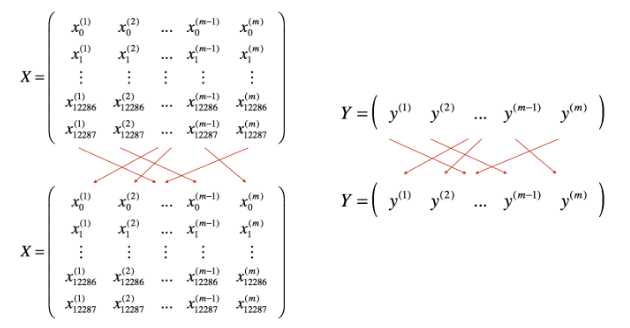
2)Partition,即把数据集分成多个大小相等batches,由于数据集大小可能不被batch size整除,所以最后一个batch的大小可能小于batch size。
代码如下:

# GRADED FUNCTION: random_mini_batches

def random_mini_batches(X, Y, mini_batch_size = 64, seed = 0):
    """
    Creates a list of random minibatches from (X, Y)

    Arguments:
    X -- input data, of shape (input size, number of examples)
    Y -- true "label" vector (1 for blue dot / 0 for red dot), of shape (1, number of examples)
    mini_batch_size -- size of the mini-batches, integer

    Returns:
    mini_batches -- list of synchronous (mini_batch_X, mini_batch_Y)
    """

    np.random.seed(seed)            # To make your "random" minibatches the same as ours
    m = X.shape[1]                  # number of training examples
    mini_batches = []

    # Step 1: Shuffle (X, Y)
    permutation = list(np.random.permutation(m))
    shuffled_X = X[:, permutation]
    shuffled_Y = Y[:, permutation].reshape((1,m))

    # Step 2: Partition (shuffled_X, shuffled_Y). Minus the end case.
    num_complete_minibatches = math.floor(m/mini_batch_size) # number of mini batches of size mini_batch_size in your partitionning
    for k in range(0, num_complete_minibatches):
        ### START CODE HERE ### (approx. 2 lines)
        mini_batch_X = shuffled_X[:,k*mini_batch_size:(k+1)*mini_batch_size]
        mini_batch_Y = shuffled_Y[:,k*mini_batch_size : (k+1)*mini_batch_size]
        ### END CODE HERE ###
        mini_batch = (mini_batch_X, mini_batch_Y)
        mini_batches.append(mini_batch)

    # Handling the end case (last mini-batch < mini_batch_size)
    if m % mini_batch_size != 0:
        ### START CODE HERE ### (approx. 2 lines)
        mini_batch_X = shuffled_X[:,num_complete_minibatches*mini_batch_size:]
        mini_batch_Y = shuffled_Y[:,num_complete_minibatches*mini_batch_size:]
        ### END CODE HERE ###
        mini_batch = (mini_batch_X, mini_batch_Y)
        mini_batches.append(mini_batch)

    return mini_batches
二.Momentum
1.由于min-batch GD在一次迭代求梯度时,只是用了部分数据集,这就不可避免地导致了梯度出现了偏差(因为掌握的信息不足以作出最明智的选择),由此使得在梯度下降的过程中出现了轻微震荡,如下图在纵向出现了震荡,而momentum可以很好地解决这个问题。
2.momentum的核心思想就是局部加权平均,最通俗的解释就是:在求当前的梯度时,把前面一部分的梯度也考虑进来,然后通过权值计算求和,最终确定当前的梯度。与普通gradient descent的每次求梯度都是相互独立的不同,momentum对于当前的梯度加入了“经验”的元素,且如果某一轴出现了震荡,那么“正反经验”相互抵消,慢慢地梯度方向也趋于平滑,最终达到消除震荡的效果。
3.那如何用数学表达式去实现momentum呢?如下:
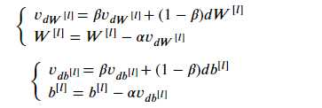
这里引入了v变量,即velocity速度的缩写。那么这个变量与速度又有什么关联?这里或许可以用物理的思想去考虑:dW就是加速度、vdW就是速度。由第一条式子可知,vdW的当前值受到原始速度vdW和加速度dW的加权影响,这样vdW就综合了两者的因素。然后在看第二个式子:W减去学习率乘以vdW,而vdW就是“过往经验”和“当前情况”的综合考虑。
代码如下(v可初始化为0,超级参数 β 一般设置为0.9):
# GRADED FUNCTION: update_parameters_with_momentum

def update_parameters_with_momentum(parameters, grads, v, beta, learning_rate):
    """
    Update parameters using Momentum

    Arguments:
    parameters -- python dictionary containing your parameters:
                    parameters[‘W‘ + str(l)] = Wl
                    parameters[‘b‘ + str(l)] = bl
    grads -- python dictionary containing your gradients for each parameters:
                    grads[‘dW‘ + str(l)] = dWl
                    grads[‘db‘ + str(l)] = dbl
    v -- python dictionary containing the current velocity:
                    v[‘dW‘ + str(l)] = ...
                    v[‘db‘ + str(l)] = ...
    beta -- the momentum hyperparameter, scalar
    learning_rate -- the learning rate, scalar

    Returns:
    parameters -- python dictionary containing your updated parameters
    v -- python dictionary containing your updated velocities
    """

    L = len(parameters) // 2 # number of layers in the neural networks

    # Momentum update for each parameter
    for l in range(L):

        ### START CODE HERE ### (approx. 4 lines)
        # compute velocities
        v["dW" + str(l+1)] = beta * v["dW" + str(l+1)] + (1-beta) * grads["dW" + str(l+1)]
        v["db" + str(l+1)] = beta * v["db" + str(l+1)] + (1-beta) * grads["db" + str(l+1)]
        # update parameters
        parameters["W" + str(l+1)] = parameters["W" + str(l+1)] - learning_rate * v["dW" + str(l+1)]
        parameters["b" + str(l+1)] = parameters["b" + str(l+1)] - learning_rate * v["db" + str(l+1)]
        ### END CODE HERE ###

    return parameters, v
3.局部加权平均有一个问题,细看表达式:![]() ,一般地v初始化为0,β初始化为0.9,所以v一开始是非常小的,要到后面才进入轨道,为了解决这个问题,需要引入修正:即再计算完
,一般地v初始化为0,β初始化为0.9,所以v一开始是非常小的,要到后面才进入轨道,为了解决这个问题,需要引入修正:即再计算完![]() 之后,v还有除以一个系数(1-β^t),即 v = v / (1-β^t),其中t是当前迭代次数。一开始时β^t小于1但接近于1,于是(1-β^t)就是一个比较小的数,v除以它之后,就能够增大数值,随着迭代次数t的增加β^t接近于0,v / (1-β^t) 就约等于v / 1,即在v进入轨道之后,修正就不再其作用,从而起到对前面的值有修正的作用。
之后,v还有除以一个系数(1-β^t),即 v = v / (1-β^t),其中t是当前迭代次数。一开始时β^t小于1但接近于1,于是(1-β^t)就是一个比较小的数,v除以它之后,就能够增大数值,随着迭代次数t的增加β^t接近于0,v / (1-β^t) 就约等于v / 1,即在v进入轨道之后,修正就不再其作用,从而起到对前面的值有修正的作用。
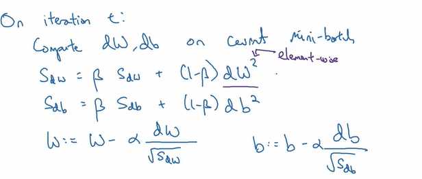
四.RMSprop
momentum解决震荡的问题,但是所谓精益求精,我们想在距离长的一方向轴上加速,在距离短的一方向轴上减速:
五.Adam
Adam则是moment和RMSprop的综合(且加入了修正),即能避免震荡,又能自动调速。其数学表达是:
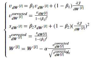
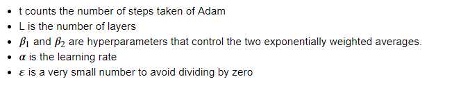
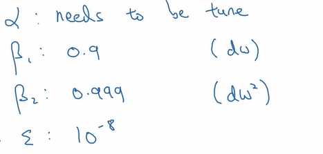
对于上面的几个超级参数,一般如下设置:
初始化v、s(一般初始化为0):
# GRADED FUNCTION: initialize_adam

def initialize_adam(parameters) :
    """
    Initializes v and s as two python dictionaries with:
                - keys: "dW1", "db1", ..., "dWL", "dbL"
                - values: numpy arrays of zeros of the same shape as the corresponding gradients/parameters.

    Arguments:
    parameters -- python dictionary containing your parameters.
                    parameters["W" + str(l)] = Wl
                    parameters["b" + str(l)] = bl

    Returns:
    v -- python dictionary that will contain the exponentially weighted average of the gradient.
                    v["dW" + str(l)] = ...
                    v["db" + str(l)] = ...
    s -- python dictionary that will contain the exponentially weighted average of the squared gradient.
                    s["dW" + str(l)] = ...
                    s["db" + str(l)] = ...

    """

    L = len(parameters) // 2 # number of layers in the neural networks
    v = {}
    s = {}

    # Initialize v, s. Input: "parameters". Outputs: "v, s".
    for l in range(L):
    ### START CODE HERE ### (approx. 4 lines)
        v["dW" + str(l+1)] = np.zeros( parameters["W" + str(l+1)].shape)
        v["db" + str(l+1)] = np.zeros( parameters["b" + str(l+1)].shape)
        s["dW" + str(l+1)] = np.zeros( parameters["W" + str(l+1)].shape)
        s["db" + str(l+1)] = np.zeros( parameters["b" + str(l+1)].shape)
    ### END CODE HERE ###

    return v, s
Adam更新参数:
# GRADED FUNCTION: update_parameters_with_adam

def update_parameters_with_adam(parameters, grads, v, s, t, learning_rate = 0.01,
                                beta1 = 0.9, beta2 = 0.999,  epsilon = 1e-8):
    """
    Update parameters using Adam

    Arguments:
    parameters -- python dictionary containing your parameters:
                    parameters[‘W‘ + str(l)] = Wl
                    parameters[‘b‘ + str(l)] = bl
    grads -- python dictionary containing your gradients for each parameters:
                    grads[‘dW‘ + str(l)] = dWl
                    grads[‘db‘ + str(l)] = dbl
    v -- Adam variable, moving average of the first gradient, python dictionary
    s -- Adam variable, moving average of the squared gradient, python dictionary
    learning_rate -- the learning rate, scalar.
    beta1 -- Exponential decay hyperparameter for the first moment estimates
    beta2 -- Exponential decay hyperparameter for the second moment estimates
    epsilon -- hyperparameter preventing division by zero in Adam updates

    Returns:
    parameters -- python dictionary containing your updated parameters
    v -- Adam variable, moving average of the first gradient, python dictionary
    s -- Adam variable, moving average of the squared gradient, python dictionary
    """

    L = len(parameters) // 2                 # number of layers in the neural networks
    v_corrected = {}                         # Initializing first moment estimate, python dictionary
    s_corrected = {}                         # Initializing second moment estimate, python dictionary

    # Perform Adam update on all parameters
    for l in range(L):
        # Moving average of the gradients. Inputs: "v, grads, beta1". Output: "v".
        ### START CODE HERE ### (approx. 2 lines)
        v["dW" + str(l+1)] = beta1 * v["dW" + str(l+1)] + (1-beta1) * grads["dW" + str(l+1)]
        v["db" + str(l+1)] = beta1 * v["db" + str(l+1)] + (1-beta1) * grads["db" + str(l+1)]
        ### END CODE HERE ###

        # Compute bias-corrected first moment estimate. Inputs: "v, beta1, t". Output: "v_corrected".
        ### START CODE HERE ### (approx. 2 lines)
        v_corrected["dW" + str(l+1)] = v["dW" + str(l+1)]/(1-beta1**t)
        v_corrected["db" + str(l+1)] = v["db" + str(l+1)]/(1-beta1**t)
        ### END CODE HERE ###

        # Moving average of the squared gradients. Inputs: "s, grads, beta2". Output: "s".
        ### START CODE HERE ### (approx. 2 lines)
        s["dW" + str(l+1)] = beta2 * s["dW" + str(l+1)] + (1-beta2) * grads["dW" + str(l+1)]**2
        s["db" + str(l+1)] = beta2 * s["db" + str(l+1)] + (1-beta2) * grads["db" + str(l+1)]**2
        ### END CODE HERE ###

        # Compute bias-corrected second raw moment estimate. Inputs: "s, beta2, t". Output: "s_corrected".
        ### START CODE HERE ### (approx. 2 lines)
        s_corrected["dW" + str(l+1)] = s["dW" + str(l+1)]/(1-beta2**t)
        s_corrected["db" + str(l+1)] = s["db" + str(l+1)]/(1-beta2**t)
        ### END CODE HERE ###

        # Update parameters. Inputs: "parameters, learning_rate, v_corrected, s_corrected, epsilon". Output: "parameters".
        ### START CODE HERE ### (approx. 2 lines)
        parameters["W" + str(l+1)] = parameters["W" + str(l+1)] - learning_rate * v_corrected["dW" + str(l+1)]/(s_corrected["dW" + str(l+1)]+epsilon)**0.5
        parameters["b" + str(l+1)] = parameters["b" + str(l+1)] - learning_rate * v_corrected["db" + str(l+1)]/(s_corrected["db" + str(l+1)]+epsilon)**0.5
        ### END CODE HERE ###

    return parameters, v, s
六.优化算法性能比较
接下来分别用mini-batch gradient descent 、 momentum 、 Adam 来对模型进行训练,并比较三者的性能。
模型如下(需要接收一个参数更新的方式):
# GRADED FUNCTION: update_parameters_with_adam

def update_parameters_with_adam(parameters, grads, v, s, t, learning_rate = 0.01,
                                beta1 = 0.9, beta2 = 0.999,  epsilon = 1e-8):
    """
    Update parameters using Adam

    Arguments:
    parameters -- python dictionary containing your parameters:
                    parameters[‘W‘ + str(l)] = Wl
                    parameters[‘b‘ + str(l)] = bl
    grads -- python dictionary containing your gradients for each parameters:
                    grads[‘dW‘ + str(l)] = dWl
                    grads[‘db‘ + str(l)] = dbl
    v -- Adam variable, moving average of the first gradient, python dictionary
    s -- Adam variable, moving average of the squared gradient, python dictionary
    learning_rate -- the learning rate, scalar.
    beta1 -- Exponential decay hyperparameter for the first moment estimates
    beta2 -- Exponential decay hyperparameter for the second moment estimates
    epsilon -- hyperparameter preventing division by zero in Adam updates

    Returns:
    parameters -- python dictionary containing your updated parameters
    v -- Adam variable, moving average of the first gradient, python dictionary
    s -- Adam variable, moving average of the squared gradient, python dictionary
    """

    L = len(parameters) // 2                 # number of layers in the neural networks
    v_corrected = {}                         # Initializing first moment estimate, python dictionary
    s_corrected = {}                         # Initializing second moment estimate, python dictionary

    # Perform Adam update on all parameters
    for l in range(L):
        # Moving average of the gradients. Inputs: "v, grads, beta1". Output: "v".
        ### START CODE HERE ### (approx. 2 lines)
        v["dW" + str(l+1)] = beta1 * v["dW" + str(l+1)] + (1-beta1) * grads["dW" + str(l+1)]
        v["db" + str(l+1)] = beta1 * v["db" + str(l+1)] + (1-beta1) * grads["db" + str(l+1)]
        ### END CODE HERE ###

        # Compute bias-corrected first moment estimate. Inputs: "v, beta1, t". Output: "v_corrected".
        ### START CODE HERE ### (approx. 2 lines)
        v_corrected["dW" + str(l+1)] = v["dW" + str(l+1)]/(1-beta1**t)
        v_corrected["db" + str(l+1)] = v["db" + str(l+1)]/(1-beta1**t)
        ### END CODE HERE ###

        # Moving average of the squared gradients. Inputs: "s, grads, beta2". Output: "s".
        ### START CODE HERE ### (approx. 2 lines)
        s["dW" + str(l+1)] = beta2 * s["dW" + str(l+1)] + (1-beta2) * grads["dW" + str(l+1)]**2
        s["db" + str(l+1)] = beta2 * s["db" + str(l+1)] + (1-beta2) * grads["db" + str(l+1)]**2
        ### END CODE HERE ###

        # Compute bias-corrected second raw moment estimate. Inputs: "s, beta2, t". Output: "s_corrected".
        ### START CODE HERE ### (approx. 2 lines)
        s_corrected["dW" + str(l+1)] = s["dW" + str(l+1)]/(1-beta2**t)
        s_corrected["db" + str(l+1)] = s["db" + str(l+1)]/(1-beta2**t)
        ### END CODE HERE ###

        # Update parameters. Inputs: "parameters, learning_rate, v_corrected, s_corrected, epsilon". Output: "parameters".
        ### START CODE HERE ### (approx. 2 lines)
        parameters["W" + str(l+1)] = parameters["W" + str(l+1)] - learning_rate * v_corrected["dW" + str(l+1)]/(s_corrected["dW" + str(l+1)]+epsilon)**0.5
        parameters["b" + str(l+1)] = parameters["b" + str(l+1)] - learning_rate * v_corrected["db" + str(l+1)]/(s_corrected["db" + str(l+1)]+epsilon)**0.5
        ### END CODE HERE ###

    return parameters, v, s
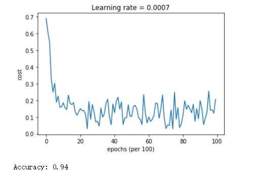
1)mini-batch gradient descent
可见其代价函数抖动得比较厉害,可能这是“mini-batch”这种选取部分数据的方式所无法避免的吧。而且准确率也不高。
2)momentum
momentum居然跟mini-batch gradient descent 的效果无异,在进行理论解释时明明是那么的美好,为什么会这样?

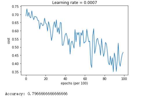
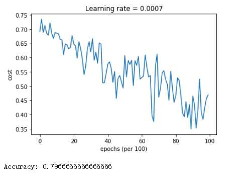
3)Adam
Adam不仅收敛速度快,而且震荡也较之不明显,更重要的是准确率高,性能明显优于mini-batch gradient descent 、 momentum。由此可见,在梯度下降的优化算法方面,Adam做得十分出色!
原文:https://www.cnblogs.com/DOLFAMINGO/p/9740843.html
