PCA主成分分析,无监督学习降维方法:
import matplotlib.pyplot as plt
import matplotlib.image as maping
import matplotlib
import numpy as np
import seaborn as sns
import pandas as pds
import plotly.graph_objs as go
import plotly.tools as tls
%matplotlib inline

from sklearn.manifold import TSNE
from sklearn.decomposition import PCA
from sklearn.discriminant_analysis import LinearDiscriminantAnalysis as LDA
使用sklearn方式展现PCA
train=pds.read_csv("train.csv")
train.head()
| label | pixel0 | pixel1 | pixel2 | pixel3 | pixel4 | pixel5 | pixel6 | pixel7 | pixel8 | pixel9 | pixel10 | pixel11 | pixel12 | pixel13 | pixel14 | pixel15 | pixel16 | pixel17 | pixel18 | pixel19 | pixel20 | pixel21 | pixel22 | pixel23 | pixel24 | pixel25 | pixel26 | pixel27 | pixel28 | pixel29 | pixel30 | pixel31 | pixel32 | pixel33 | pixel34 | pixel35 | pixel36 | pixel37 | pixel38 | pixel39 | pixel40 | pixel41 | pixel42 | pixel43 | pixel44 | pixel45 | pixel46 | pixel47 | pixel48 | pixel49 | pixel50 | pixel51 | pixel52 | pixel53 | pixel54 | pixel55 | pixel56 | pixel57 | pixel58 | ... | pixel724 | pixel725 | pixel726 | pixel727 | pixel728 | pixel729 | pixel730 | pixel731 | pixel732 | pixel733 | pixel734 | pixel735 | pixel736 | pixel737 | pixel738 | pixel739 | pixel740 | pixel741 | pixel742 | pixel743 | pixel744 | pixel745 | pixel746 | pixel747 | pixel748 | pixel749 | pixel750 | pixel751 | pixel752 | pixel753 | pixel754 | pixel755 | pixel756 | pixel757 | pixel758 | pixel759 | pixel760 | pixel761 | pixel762 | pixel763 | pixel764 | pixel765 | pixel766 | pixel767 | pixel768 | pixel769 | pixel770 | pixel771 | pixel772 | pixel773 | pixel774 | pixel775 | pixel776 | pixel777 | pixel778 | pixel779 | pixel780 | pixel781 | pixel782 | pixel783 | |
|---|---|---|---|---|---|---|---|---|---|---|---|---|---|---|---|---|---|---|---|---|---|---|---|---|---|---|---|---|---|---|---|---|---|---|---|---|---|---|---|---|---|---|---|---|---|---|---|---|---|---|---|---|---|---|---|---|---|---|---|---|---|---|---|---|---|---|---|---|---|---|---|---|---|---|---|---|---|---|---|---|---|---|---|---|---|---|---|---|---|---|---|---|---|---|---|---|---|---|---|---|---|---|---|---|---|---|---|---|---|---|---|---|---|---|---|---|---|---|---|---|---|
| 0 | 1 | 0 | 0 | 0 | 0 | 0 | 0 | 0 | 0 | 0 | 0 | 0 | 0 | 0 | 0 | 0 | 0 | 0 | 0 | 0 | 0 | 0 | 0 | 0 | 0 | 0 | 0 | 0 | 0 | 0 | 0 | 0 | 0 | 0 | 0 | 0 | 0 | 0 | 0 | 0 | 0 | 0 | 0 | 0 | 0 | 0 | 0 | 0 | 0 | 0 | 0 | 0 | 0 | 0 | 0 | 0 | 0 | 0 | 0 | 0 | ... | 0 | 0 | 0 | 0 | 0 | 0 | 0 | 0 | 0 | 0 | 0 | 0 | 0 | 0 | 0 | 0 | 0 | 0 | 0 | 0 | 0 | 0 | 0 | 0 | 0 | 0 | 0 | 0 | 0 | 0 | 0 | 0 | 0 | 0 | 0 | 0 | 0 | 0 | 0 | 0 | 0 | 0 | 0 | 0 | 0 | 0 | 0 | 0 | 0 | 0 | 0 | 0 | 0 | 0 | 0 | 0 | 0 | 0 | 0 | 0 |
| 1 | 0 | 0 | 0 | 0 | 0 | 0 | 0 | 0 | 0 | 0 | 0 | 0 | 0 | 0 | 0 | 0 | 0 | 0 | 0 | 0 | 0 | 0 | 0 | 0 | 0 | 0 | 0 | 0 | 0 | 0 | 0 | 0 | 0 | 0 | 0 | 0 | 0 | 0 | 0 | 0 | 0 | 0 | 0 | 0 | 0 | 0 | 0 | 0 | 0 | 0 | 0 | 0 | 0 | 0 | 0 | 0 | 0 | 0 | 0 | 0 | ... | 0 | 0 | 0 | 0 | 0 | 0 | 0 | 0 | 0 | 0 | 0 | 0 | 0 | 0 | 0 | 0 | 0 | 0 | 0 | 0 | 0 | 0 | 0 | 0 | 0 | 0 | 0 | 0 | 0 | 0 | 0 | 0 | 0 | 0 | 0 | 0 | 0 | 0 | 0 | 0 | 0 | 0 | 0 | 0 | 0 | 0 | 0 | 0 | 0 | 0 | 0 | 0 | 0 | 0 | 0 | 0 | 0 | 0 | 0 | 0 |
| 2 | 1 | 0 | 0 | 0 | 0 | 0 | 0 | 0 | 0 | 0 | 0 | 0 | 0 | 0 | 0 | 0 | 0 | 0 | 0 | 0 | 0 | 0 | 0 | 0 | 0 | 0 | 0 | 0 | 0 | 0 | 0 | 0 | 0 | 0 | 0 | 0 | 0 | 0 | 0 | 0 | 0 | 0 | 0 | 0 | 0 | 0 | 0 | 0 | 0 | 0 | 0 | 0 | 0 | 0 | 0 | 0 | 0 | 0 | 0 | 0 | ... | 0 | 0 | 0 | 0 | 0 | 0 | 0 | 0 | 0 | 0 | 0 | 0 | 0 | 0 | 0 | 0 | 0 | 0 | 0 | 0 | 0 | 0 | 0 | 0 | 0 | 0 | 0 | 0 | 0 | 0 | 0 | 0 | 0 | 0 | 0 | 0 | 0 | 0 | 0 | 0 | 0 | 0 | 0 | 0 | 0 | 0 | 0 | 0 | 0 | 0 | 0 | 0 | 0 | 0 | 0 | 0 | 0 | 0 | 0 | 0 |
| 3 | 4 | 0 | 0 | 0 | 0 | 0 | 0 | 0 | 0 | 0 | 0 | 0 | 0 | 0 | 0 | 0 | 0 | 0 | 0 | 0 | 0 | 0 | 0 | 0 | 0 | 0 | 0 | 0 | 0 | 0 | 0 | 0 | 0 | 0 | 0 | 0 | 0 | 0 | 0 | 0 | 0 | 0 | 0 | 0 | 0 | 0 | 0 | 0 | 0 | 0 | 0 | 0 | 0 | 0 | 0 | 0 | 0 | 0 | 0 | 0 | ... | 0 | 0 | 0 | 0 | 0 | 0 | 0 | 0 | 0 | 0 | 0 | 0 | 0 | 0 | 0 | 0 | 0 | 0 | 0 | 0 | 0 | 0 | 0 | 0 | 0 | 0 | 0 | 0 | 0 | 0 | 0 | 0 | 0 | 0 | 0 | 0 | 0 | 0 | 0 | 0 | 0 | 0 | 0 | 0 | 0 | 0 | 0 | 0 | 0 | 0 | 0 | 0 | 0 | 0 | 0 | 0 | 0 | 0 | 0 | 0 |
| 4 | 0 | 0 | 0 | 0 | 0 | 0 | 0 | 0 | 0 | 0 | 0 | 0 | 0 | 0 | 0 | 0 | 0 | 0 | 0 | 0 | 0 | 0 | 0 | 0 | 0 | 0 | 0 | 0 | 0 | 0 | 0 | 0 | 0 | 0 | 0 | 0 | 0 | 0 | 0 | 0 | 0 | 0 | 0 | 0 | 0 | 0 | 0 | 0 | 0 | 0 | 0 | 0 | 0 | 0 | 0 | 0 | 0 | 0 | 0 | 0 | ... | 0 | 0 | 0 | 0 | 0 | 0 | 0 | 0 | 0 | 0 | 0 | 0 | 0 | 0 | 0 | 0 | 0 | 0 | 0 | 0 | 0 | 0 | 0 | 0 | 0 | 0 | 0 | 0 | 0 | 0 | 0 | 0 | 0 | 0 | 0 | 0 | 0 | 0 | 0 | 0 | 0 | 0 | 0 | 0 | 0 | 0 | 0 | 0 | 0 | 0 | 0 | 0 | 0 | 0 | 0 | 0 | 0 | 0 | 0 | 0 |
print(train.shape)
target=train["label"]
train=train.drop("label",axis=1)
train.head()
| pixel0 | pixel1 | pixel2 | pixel3 | pixel4 | pixel5 | pixel6 | pixel7 | pixel8 | pixel9 | pixel10 | pixel11 | pixel12 | pixel13 | pixel14 | pixel15 | pixel16 | pixel17 | pixel18 | pixel19 | pixel20 | pixel21 | pixel22 | pixel23 | pixel24 | pixel25 | pixel26 | pixel27 | pixel28 | pixel29 | pixel30 | pixel31 | pixel32 | pixel33 | pixel34 | pixel35 | pixel36 | pixel37 | pixel38 | pixel39 | pixel40 | pixel41 | pixel42 | pixel43 | pixel44 | pixel45 | pixel46 | pixel47 | pixel48 | pixel49 | pixel50 | pixel51 | pixel52 | pixel53 | pixel54 | pixel55 | pixel56 | pixel57 | pixel58 | pixel59 | ... | pixel724 | pixel725 | pixel726 | pixel727 | pixel728 | pixel729 | pixel730 | pixel731 | pixel732 | pixel733 | pixel734 | pixel735 | pixel736 | pixel737 | pixel738 | pixel739 | pixel740 | pixel741 | pixel742 | pixel743 | pixel744 | pixel745 | pixel746 | pixel747 | pixel748 | pixel749 | pixel750 | pixel751 | pixel752 | pixel753 | pixel754 | pixel755 | pixel756 | pixel757 | pixel758 | pixel759 | pixel760 | pixel761 | pixel762 | pixel763 | pixel764 | pixel765 | pixel766 | pixel767 | pixel768 | pixel769 | pixel770 | pixel771 | pixel772 | pixel773 | pixel774 | pixel775 | pixel776 | pixel777 | pixel778 | pixel779 | pixel780 | pixel781 | pixel782 | pixel783 | |
|---|---|---|---|---|---|---|---|---|---|---|---|---|---|---|---|---|---|---|---|---|---|---|---|---|---|---|---|---|---|---|---|---|---|---|---|---|---|---|---|---|---|---|---|---|---|---|---|---|---|---|---|---|---|---|---|---|---|---|---|---|---|---|---|---|---|---|---|---|---|---|---|---|---|---|---|---|---|---|---|---|---|---|---|---|---|---|---|---|---|---|---|---|---|---|---|---|---|---|---|---|---|---|---|---|---|---|---|---|---|---|---|---|---|---|---|---|---|---|---|---|---|
| 0 | 0 | 0 | 0 | 0 | 0 | 0 | 0 | 0 | 0 | 0 | 0 | 0 | 0 | 0 | 0 | 0 | 0 | 0 | 0 | 0 | 0 | 0 | 0 | 0 | 0 | 0 | 0 | 0 | 0 | 0 | 0 | 0 | 0 | 0 | 0 | 0 | 0 | 0 | 0 | 0 | 0 | 0 | 0 | 0 | 0 | 0 | 0 | 0 | 0 | 0 | 0 | 0 | 0 | 0 | 0 | 0 | 0 | 0 | 0 | 0 | ... | 0 | 0 | 0 | 0 | 0 | 0 | 0 | 0 | 0 | 0 | 0 | 0 | 0 | 0 | 0 | 0 | 0 | 0 | 0 | 0 | 0 | 0 | 0 | 0 | 0 | 0 | 0 | 0 | 0 | 0 | 0 | 0 | 0 | 0 | 0 | 0 | 0 | 0 | 0 | 0 | 0 | 0 | 0 | 0 | 0 | 0 | 0 | 0 | 0 | 0 | 0 | 0 | 0 | 0 | 0 | 0 | 0 | 0 | 0 | 0 |
| 1 | 0 | 0 | 0 | 0 | 0 | 0 | 0 | 0 | 0 | 0 | 0 | 0 | 0 | 0 | 0 | 0 | 0 | 0 | 0 | 0 | 0 | 0 | 0 | 0 | 0 | 0 | 0 | 0 | 0 | 0 | 0 | 0 | 0 | 0 | 0 | 0 | 0 | 0 | 0 | 0 | 0 | 0 | 0 | 0 | 0 | 0 | 0 | 0 | 0 | 0 | 0 | 0 | 0 | 0 | 0 | 0 | 0 | 0 | 0 | 0 | ... | 0 | 0 | 0 | 0 | 0 | 0 | 0 | 0 | 0 | 0 | 0 | 0 | 0 | 0 | 0 | 0 | 0 | 0 | 0 | 0 | 0 | 0 | 0 | 0 | 0 | 0 | 0 | 0 | 0 | 0 | 0 | 0 | 0 | 0 | 0 | 0 | 0 | 0 | 0 | 0 | 0 | 0 | 0 | 0 | 0 | 0 | 0 | 0 | 0 | 0 | 0 | 0 | 0 | 0 | 0 | 0 | 0 | 0 | 0 | 0 |
| 2 | 0 | 0 | 0 | 0 | 0 | 0 | 0 | 0 | 0 | 0 | 0 | 0 | 0 | 0 | 0 | 0 | 0 | 0 | 0 | 0 | 0 | 0 | 0 | 0 | 0 | 0 | 0 | 0 | 0 | 0 | 0 | 0 | 0 | 0 | 0 | 0 | 0 | 0 | 0 | 0 | 0 | 0 | 0 | 0 | 0 | 0 | 0 | 0 | 0 | 0 | 0 | 0 | 0 | 0 | 0 | 0 | 0 | 0 | 0 | 0 | ... | 0 | 0 | 0 | 0 | 0 | 0 | 0 | 0 | 0 | 0 | 0 | 0 | 0 | 0 | 0 | 0 | 0 | 0 | 0 | 0 | 0 | 0 | 0 | 0 | 0 | 0 | 0 | 0 | 0 | 0 | 0 | 0 | 0 | 0 | 0 | 0 | 0 | 0 | 0 | 0 | 0 | 0 | 0 | 0 | 0 | 0 | 0 | 0 | 0 | 0 | 0 | 0 | 0 | 0 | 0 | 0 | 0 | 0 | 0 | 0 |
| 3 | 0 | 0 | 0 | 0 | 0 | 0 | 0 | 0 | 0 | 0 | 0 | 0 | 0 | 0 | 0 | 0 | 0 | 0 | 0 | 0 | 0 | 0 | 0 | 0 | 0 | 0 | 0 | 0 | 0 | 0 | 0 | 0 | 0 | 0 | 0 | 0 | 0 | 0 | 0 | 0 | 0 | 0 | 0 | 0 | 0 | 0 | 0 | 0 | 0 | 0 | 0 | 0 | 0 | 0 | 0 | 0 | 0 | 0 | 0 | 0 | ... | 0 | 0 | 0 | 0 | 0 | 0 | 0 | 0 | 0 | 0 | 0 | 0 | 0 | 0 | 0 | 0 | 0 | 0 | 0 | 0 | 0 | 0 | 0 | 0 | 0 | 0 | 0 | 0 | 0 | 0 | 0 | 0 | 0 | 0 | 0 | 0 | 0 | 0 | 0 | 0 | 0 | 0 | 0 | 0 | 0 | 0 | 0 | 0 | 0 | 0 | 0 | 0 | 0 | 0 | 0 | 0 | 0 | 0 | 0 | 0 |
| 4 | 0 | 0 | 0 | 0 | 0 | 0 | 0 | 0 | 0 | 0 | 0 | 0 | 0 | 0 | 0 | 0 | 0 | 0 | 0 | 0 | 0 | 0 | 0 | 0 | 0 | 0 | 0 | 0 | 0 | 0 | 0 | 0 | 0 | 0 | 0 | 0 | 0 | 0 | 0 | 0 | 0 | 0 | 0 | 0 | 0 | 0 | 0 | 0 | 0 | 0 | 0 | 0 | 0 | 0 | 0 | 0 | 0 | 0 | 0 | 0 | ... | 0 | 0 | 0 | 0 | 0 | 0 | 0 | 0 | 0 | 0 | 0 | 0 | 0 | 0 | 0 | 0 | 0 | 0 | 0 | 0 | 0 | 0 | 0 | 0 | 0 | 0 | 0 | 0 | 0 | 0 | 0 | 0 | 0 | 0 | 0 | 0 | 0 | 0 | 0 | 0 | 0 | 0 | 0 | 0 | 0 | 0 | 0 | 0 | 0 | 0 | 0 | 0 | 0 | 0 | 0 | 0 | 0 | 0 | 0 | 0 |
#数据标准化
from sklearn.preprocessing import StandardScaler
X=train.values
transform=StandardScaler()
X_std=transform.fit_transform(X)

c:\users\lenovo\appdata\local\programs\python\python36\lib\site-packages\sklearn\utils\validation.py:595: DataConversionWarning:

Data with input dtype int64 was converted to float64 by StandardScaler.

c:\users\lenovo\appdata\local\programs\python\python36\lib\site-packages\sklearn\utils\validation.py:595: DataConversionWarning:

Data with input dtype int64 was converted to float64 by StandardScaler.
#特征向量和特征值
mean_vec=np.mean(X_std,axis=0)
cov_mat=np.cov(X_std.T)
eig_vals,eig_vecs=np.linalg.eig(cov_mat)
#创建特征向量和特征值的元组
eig_pairs=[(np.abs(eig_vals[i]),eig_vecs[:,i] for i in range(len(eig_vals))]
#对特征向量和特征值进行排序
eig_pairs.sort(key=lambda x : x[0],reverse=True)
#计算累计解释方差
tot=sum(eig_vals)
var_exp=[(i/tot)*100 for i  in sorted(eig_vals,reverse=True)]
cum_var_exp=np.cumsum(var_exp)
#接下来使用Ploty可视化显示
trace1=go.Scatter(x=list(range(784)),y=cum_var_exp,mode="lines+markers",name="‘累计解释方差‘",line=dict(shape=‘spline‘,color=‘goldenrod‘))
trace2=go.Scatter(x=list(range(784)),y=var_exp,mode="lines+markers",name="‘单个解释方差‘",line=dict(shape=‘linear‘,color=‘black‘))
fig=tls.make_subplots(insets=[{‘cell‘:(1,1),‘l‘:0.7,‘b‘:0.5}],print_grid=True)
fig.append_trace(trace1,1,1)
fig.append_trace(trace2,1,1)
fig.layout.title="解释方差"
fig.layout.xaxis=dict(range=[0,80],title="特征列")
fig.layout.yaxis=dict(range=[0,60],title="解释变量")
This is the format of your plot grid:
[ (1,1) x1,y1 ]

With insets:
[ x2,y2 ] over [ (1,1) x1,y1 ]
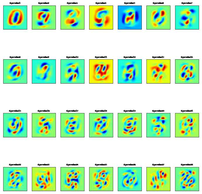
#可视化特征值
n_components=30
pca=PCA(n_components=n_components).fit(train.values)
eigenvalues=pca.components_.reshape(n_components,28,28)
eigenvalues=pca.components_
n_row=4
n_col=7

#显示前8个特征值
plt.figure(figsize=(12,13))
for i in list(range(n_row*n_col)):
    offset=0
    plt.subplot(n_row,n_col,i+1)
    plt.imshow(eigenvalues[i].reshape(28,28),cmap=‘jet‘)
    title_text="Eigenvalue"+str(i+1)
    plt.title(title_text,size=6.5)
    plt.xticks(())
    plt.yticks(())
plt.show()
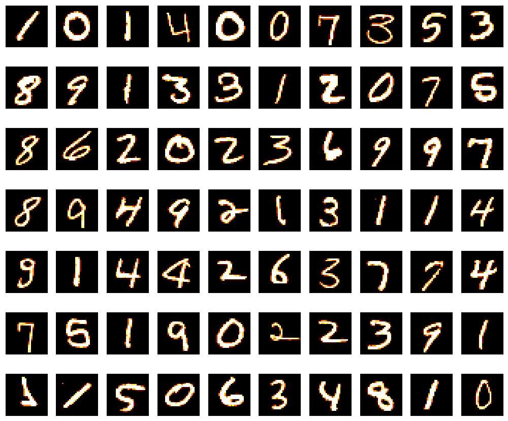
plt.figure(figsize=(14,12))
for digit_num in range(0,70):
    plt.subplot(7,10,digit_num+1)
    grid_data=train.iloc[digit_num].as_matrix().reshape(28,28)
    plt.imshow(grid_data,interpolation="none",cmap="afmhot")
    plt.xticks([])
    plt.yticks([])
plt.tight_layout()
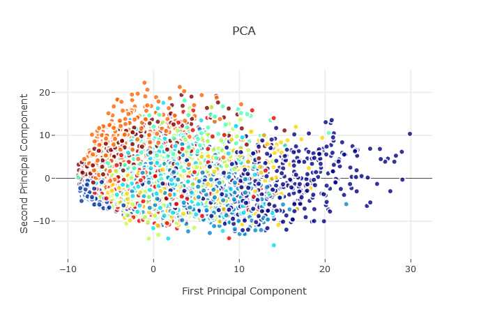
#PCA使用在SK-learn中
del X
X=train[:6000].values
del train
X_std=StandardScaler().fit_transform(X)
pca=PCA(n_components=5)
pca.fit(X_std)
X_5d=pca.transform(X_std)
#使用散点图显示PCA效果
import plotly.offline as py
py.offline.init_notebook_mode(connected=True)
Target=target[:6000]
trace0=go.Scatter(x=X_5d[:,0],y=X_5d[:,1],mode="markers",text=Target,showlegend=False,marker=dict(size=8,color=Target,colorscale="Jet",showscale=False,line=dict(width=2,color="rgb(255,255,255)"),opacity=0.8))
data=[trace0]
layout=go.Layout(title="PCA",hovermode="closest",xaxis=dict(title="First Principal Component",ticklen=5,zeroline=False,gridwidth=2,),yaxis=dict(title="Second Principal Component",ticklen=5,gridwidth=2,),showlegend=True)
fig=dict(data=data,layout=layout)
py.iplot(fig,filename="style-scatter")
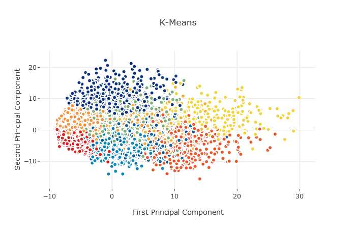
from sklearn.cluster import KMeans
kmeans=KMeans(n_clusters=9)
X_clustered=kmeans.fit_predict(X_5d)
trace_Kmeans=go.Scatter(x=X_5d[:,0],y=X_5d[:,1],mode="markers",showlegend=False,marker=dict(size=8,color=X_clustered,colorscale="Portland",showscale=False,line=dict(width=2,color=‘rgb(255,255,255)‘)))
layout=go.Layout(title="K-Means",hovermode="closest",xaxis=dict(title="First Principal Component",ticklen=5,zeroline=False,gridwidth=2,),yaxis=dict(title="Second Principal Component",ticklen=5,gridwidth=2,),showlegend=True)
data=[trace_Kmeans]
fig1=dict(data=data,layout=layout)
py.iplot(fig1,filename="svm")
原文:https://www.cnblogs.com/knight-vien/p/10433683.html