这个主要是线性回归和逻辑回归部分,除了前面关于最小二乘法,后面基本都看不懂,只做了记录。
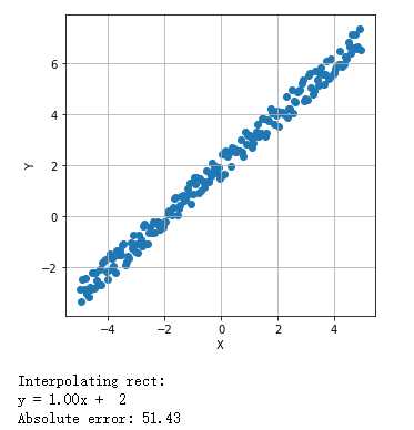
二维线性模型:普通最小二乘法:


 1 from __future__ import print_function
 2 import numpy as np
 3 import matplotlib.pyplot as plt
 4 from scipy.optimize import minimize
 5
 6 # For reproducibility
 7 np.random.seed(1000)
 8 # Number of samples
 9 nb_samples = 200
10
11 def loss(v):
12     e = 0.0
13     for i in range(nb_samples):
14         e += np.square(v[0] + v[1]*X[i] - Y[i])
15     return 0.5 * e
16
17 def gradient(v):
18     g = np.zeros(shape=2)
19     for i in range(nb_samples):
20         g[0] += (v[0] + v[1]*X[i] - Y[i])
21         g[1] += ((v[0] + v[1]*X[i] - Y[i]) * X[i])
22     return g
23
24 def show_dataset(X, Y):
25     fig, ax = plt.subplots(1, 1, figsize=(5, 5))
26     ax.scatter(X, Y)
27     ax.set_xlabel(‘X‘)
28     ax.set_ylabel(‘Y‘)
29     ax.grid()
30     plt.show()
31
32 if __name__ == ‘__main__‘:
33     # Create dataset
34     X = np.arange(-5, 5, 0.05)
35     Y = X + 2
36     Y += np.random.uniform(-0.5, 0.5, size=nb_samples)
37
38     # Show the dataset
39     show_dataset(X, Y)
40
41     # Minimize loss function
42     result = minimize(fun=loss, x0=np.array([0.0, 0.0]), jac=gradient, method=‘L-BFGS-B‘)
43
44     print(‘Interpolating rect:‘)
45     print(‘y = %.2fx + %2.f‘ % (result.x[1], result.x[0]))
46
47     # Compute the absolute error
48     err = 0.0
49
50     for i in range(nb_samples):
51         err += np.abs(Y[i] - (result.x[1]*X[i] + result.x[0]))
52
53     print(‘Absolute error: %.2f‘ % err)
基于scikit-learn的线性回归和更高维:
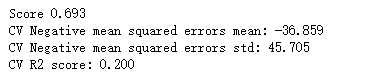
利用k折交叉验证完成测试:

在交叉验证中,使用scoring=‘r2‘时,R2接近于1效果好,接近0模型差。R2=1-(xxx/XXXXX)
 1 from __future__  import print_function
 2 import numpy as np
 3 import matplotlib.pyplot as plt
 4 from sklearn.datasets import load_boston
 5 from sklearn.linear_model import LinearRegression
 6 from sklearn.model_selection import train_test_split, cross_val_score
 7 # For reproducibility
 8 np.random.seed(1000)
 9 def show_dataset(data):
10     fig, ax = plt.subplots(4, 3, figsize=(20, 15))
11     for i in range(4):
12         for j in range(3):
13             ax[i, j].plot(data.data[:, i + (j + 1) * 3])
14             ax[i, j].grid()
15     plt.show()
16
17 if __name__ == ‘__main__‘:
18     # Load dataset
19     boston = load_boston()
20     # Show dataset
21     show_dataset(boston)
22     # Create a linear regressor instance
23     lr = LinearRegression(normalize=True)
24     # Split dataset
25     X_train, X_test, Y_train, Y_test = train_test_split(boston.data, boston.target, test_size=0.1)
26     # Train the model
27     lr.fit(X_train, Y_train)
28     print(‘Score %.3f‘ % lr.score(X_test, Y_test))
29     # CV score  k折交叉验证,负均方差验证
30     scores = cross_val_score(lr, boston.data, boston.target, cv=7, scoring=‘neg_mean_squared_error‘)
31     print(‘CV Negative mean squared errors mean: %.3f‘ % scores.mean())
32     print(‘CV Negative mean squared errors std: %.3f‘ % scores.std())
33     # CV R2 score   k折交叉验证,决定系数验证
34     r2_scores = cross_val_score(lr, boston.data, boston.target, cv=10, scoring=‘r2‘)
35     print(‘CV R2 score: %.3f‘ % r2_scores.mean())
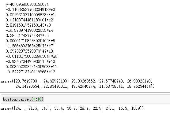
求得的回归表达式和结果:(不理想的结果)
1 print(‘y=‘+ str(lr.intercept_)+‘ ‘)
2 for i,c in enumerate(lr.coef_):
3     print(str(c)+‘*x‘+str(i))
4 X = boston.data[0:10]+np.random.normal(0.0,0.1)
5 lr.predict(X)
boston.target[0:10]
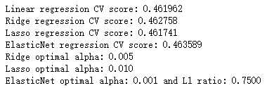
Ridge、Lasso、ElasticNet回归:
 1 from __future__ import print_function
 2 import numpy as np
 3 from sklearn.datasets import load_diabetes
 4 from sklearn.linear_model import LinearRegression, Ridge, Lasso, ElasticNet, RidgeCV, LassoCV, ElasticNetCV
 5 from sklearn.model_selection import cross_val_score
 6 # For reproducibility
 7 np.random.seed(1000)
 8 if __name__ == ‘__main__‘:
 9     diabetes = load_diabetes()
10     # Create a linear regressor and compute CV score
11     lr = LinearRegression(normalize=True)
12     lr_scores = cross_val_score(lr, diabetes.data, diabetes.target, cv=10)
13     print(‘Linear regression CV score: %.6f‘ % lr_scores.mean())
14     # Create a Ridge regressor and compute CV score
15     rg = Ridge(0.005, normalize=True)
16     rg_scores = cross_val_score(rg, diabetes.data, diabetes.target, cv=10)
17     print(‘Ridge regression CV score: %.6f‘ % rg_scores.mean())
18     # Create a Lasso regressor and compute CV score
19     ls = Lasso(0.01, normalize=True)
20     ls_scores = cross_val_score(ls, diabetes.data, diabetes.target, cv=10)
21     print(‘Lasso regression CV score: %.6f‘ % ls_scores.mean())
22     # Create ElasticNet regressor and compute CV score
23     en = ElasticNet(alpha=0.001, l1_ratio=0.8, normalize=True)
24     en_scores = cross_val_score(en, diabetes.data, diabetes.target, cv=10)
25     print(‘ElasticNet regression CV score: %.6f‘ % en_scores.mean())
26
27     # Find the optimal alpha value for Ridge regression
28     rgcv = RidgeCV(alphas=(1.0, 0.1, 0.01, 0.001, 0.005, 0.0025, 0.001, 0.00025), normalize=True)
29     rgcv.fit(diabetes.data, diabetes.target)
30     print(‘Ridge optimal alpha: %.3f‘ % rgcv.alpha_)
31     # Find the optimal alpha value for Lasso regression
32     lscv = LassoCV(alphas=(1.0, 0.1, 0.01, 0.001, 0.005, 0.0025, 0.001, 0.00025), normalize=True)
33     lscv.fit(diabetes.data, diabetes.target)
34     print(‘Lasso optimal alpha: %.3f‘ % lscv.alpha_)
35     # Find the optimal alpha and l1_ratio for Elastic Net
36     encv = ElasticNetCV(alphas=(0.1, 0.01, 0.005, 0.0025, 0.001), l1_ratio=(0.1, 0.25, 0.5, 0.75, 0.8), normalize=True)
37     encv.fit(diabetes.data, diabetes.target)
38     print(‘ElasticNet optimal alpha: %.3f and L1 ratio: %.4f‘ % (encv.alpha_, encv.l1_ratio_))
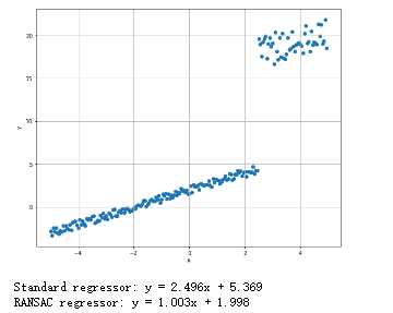
随机采样一致的鲁棒回归:
 1 from __future__ import print_function
 2 import numpy as np
 3 import matplotlib.pyplot as plt
 4 from sklearn.linear_model import LinearRegression, RANSACRegressor
 5 # For reproducibility
 6 np.random.seed(1000)
 7 nb_samples = 200
 8 nb_noise_samples = 150
 9
10 def show_dataset(X, Y):
11     fig, ax = plt.subplots(1, 1, figsize=(10, 8))
12     ax.scatter(X, Y)
13     ax.set_xlabel(‘X‘)
14     ax.set_ylabel(‘Y‘)
15     ax.grid()
16     plt.show()
17
18 if __name__ == ‘__main__‘:
19     # Create dataset
20     X = np.arange(-5, 5, 0.05)
21     Y = X + 2
22     Y += np.random.uniform(-0.5, 0.5, size=nb_samples)
23     for i in range(nb_noise_samples, nb_samples):
24         Y[i] += np.random.uniform(12, 15)
25     # Show the dataset
26     show_dataset(X, Y)
27     # Create a linear regressor
28     lr = LinearRegression(normalize=True)
29     lr.fit(X.reshape(-1, 1), Y.reshape(-1, 1))
30     print(‘Standard regressor: y = %.3fx + %.3f‘ % (lr.coef_, lr.intercept_))
31     # Create RANSAC regressor
32     rs = RANSACRegressor(lr)
33     rs.fit(X.reshape(-1, 1), Y.reshape(-1, 1))
34     print(‘RANSAC regressor: y = %.3fx + %.3f‘ % (rs.estimator_.coef_, rs.estimator_.intercept_))
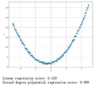
多项式回归:
 1 from __future__ import print_function
 2 import numpy as np
 3 import matplotlib.pyplot as plt
 4 from sklearn.linear_model import LinearRegression
 5 from sklearn.model_selection import train_test_split
 6 from sklearn.preprocessing import PolynomialFeatures
 7 # For reproducibility
 8 np.random.seed(1000)
 9 nb_samples = 200
10 def show_dataset(X, Y):
11     fig, ax = plt.subplots(1, 1, figsize=(10, 8))
12     ax.scatter(X, Y)
13     ax.set_xlabel(‘X‘)
14     ax.set_ylabel(‘Y‘)
15     ax.grid()
16     plt.show()
17
18 if __name__ == ‘__main__‘:
19     # Create dataset
20     X = np.arange(-5, 5, 0.05)
21     Y = X + 2
22     Y += X**2 + np.random.uniform(-0.5, 0.5, size=nb_samples)
23     # Show the dataset
24     show_dataset(X, Y)
25     # Split dataset
26     X_train, X_test, Y_train, Y_test = train_test_split(X.reshape(-1, 1), Y.reshape(-1, 1), test_size=0.25)
27     lr = LinearRegression(normalize=True)
28     lr.fit(X_train, Y_train)
29     print(‘Linear regression score: %.3f‘ % lr.score(X_train, Y_train))
30     # Create polynomial features
31     pf = PolynomialFeatures(degree=2)
32     X_train = pf.fit_transform(X_train)
33     X_test = pf.fit_transform(X_test)
34     lr.fit(X_train, Y_train)
35     print(‘Second degree polynomial regression score: %.3f‘ % lr.score(X_train, Y_train))
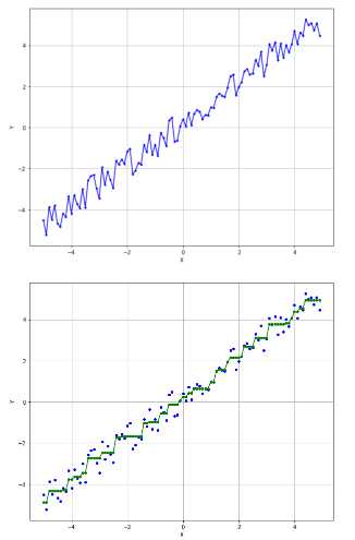
保序回归:
 1 from __future__ import print_function
 2 import numpy as np
 3 import matplotlib.pyplot as plt
 4 from matplotlib.collections import LineCollection
 5 from sklearn.isotonic import IsotonicRegression
 6 # For reproducibility
 7 np.random.seed(1000)
 8 nb_samples = 100
 9 def show_dataset(X, Y):
10     fig, ax = plt.subplots(1, 1, figsize=(10, 8))
11     ax.plot(X, Y, ‘b.-‘)
12     ax.grid()
13     ax.set_xlabel(‘X‘)
14     ax.set_ylabel(‘Y‘)
15     plt.show()
16
17 def show_isotonic_regression_segments(X, Y, Yi, segments):
18     lc = LineCollection(segments, zorder=0)
19     lc.set_array(np.ones(len(Y)))
20     lc.set_linewidths(0.5 * np.ones(nb_samples))
21     fig, ax = plt.subplots(1, 1, figsize=(10, 8))
22     ax.plot(X, Y, ‘b.‘, markersize=8)
23     ax.plot(X, Yi, ‘g.-‘, markersize=8)
24     ax.grid()
25     ax.set_xlabel(‘X‘)
26     ax.set_ylabel(‘Y‘)
27     plt.show()
28
29 if __name__ == ‘__main__‘:
30     # Create dataset
31     X = np.arange(-5, 5, 0.1)
32     Y = X + np.random.uniform(-0.5, 1, size=X.shape)
33     # Show original dataset
34     show_dataset(X, Y)
35     # Create an isotonic regressor
36     ir = IsotonicRegression(-6, 10)
37     Yi = ir.fit_transform(X, Y)
38     # Create a segment list
39     segments = [[[i, Y[i]], [i, Yi[i]]] for i in range(nb_samples)]
40     # Show isotonic interpolation
41     show_isotonic_regression_segments(X, Y, Yi, segments)
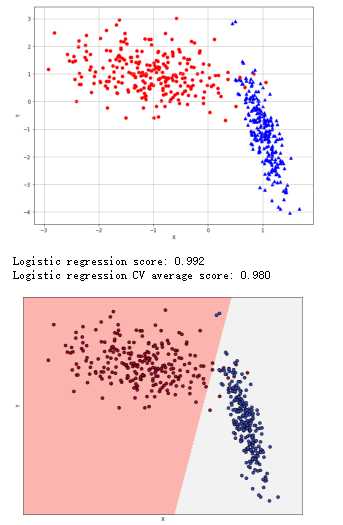
逻辑回归:
 1 from __future__ import print_function
 2 import numpy as np
 3 import matplotlib.pyplot as plt
 4 from sklearn.datasets import make_classification
 5 from sklearn.model_selection import train_test_split, cross_val_score
 6 from sklearn.linear_model import LogisticRegression
 7 # For reproducibility
 8 np.random.seed(1000)
 9 nb_samples = 500
10
11 def show_dataset(X, Y):
12     fig, ax = plt.subplots(1, 1, figsize=(10, 8))
13     ax.grid()
14     ax.set_xlabel(‘X‘)
15     ax.set_ylabel(‘Y‘)
16     for i in range(nb_samples):
17         if Y[i] == 0:
18             ax.scatter(X[i, 0], X[i, 1], marker=‘o‘, color=‘r‘)
19         else:
20             ax.scatter(X[i, 0], X[i, 1], marker=‘^‘, color=‘b‘)
21     plt.show()
22
23 def show_classification_areas(X, Y, lr):
24     x_min, x_max = X[:, 0].min() - .5, X[:, 0].max() + .5
25     y_min, y_max = X[:, 1].min() - .5, X[:, 1].max() + .5
26     xx, yy = np.meshgrid(np.arange(x_min, x_max, 0.02), np.arange(y_min, y_max, 0.02))
27     Z = lr.predict(np.c_[xx.ravel(), yy.ravel()])
28     Z = Z.reshape(xx.shape)
29     plt.figure(1, figsize=(10, 8))
30     plt.pcolormesh(xx, yy, Z, cmap=plt.cm.Pastel1)
31     # Plot also the training points
32     plt.scatter(X[:, 0], X[:, 1], c=np.abs(Y - 1), edgecolors=‘k‘, cmap=plt.cm.coolwarm)
33     plt.xlabel(‘X‘)
34     plt.ylabel(‘Y‘)
35     plt.xlim(xx.min(), xx.max())
36     plt.ylim(yy.min(), yy.max())
37     plt.xticks(())
38     plt.yticks(())
39     plt.show()
40
41 if __name__ == ‘__main__‘:
42     # Create dataset
43     X, Y = make_classification(n_samples=nb_samples, n_features=2, n_informative=2, n_redundant=0,
44                                n_clusters_per_class=1)
45     # Show dataset
46     show_dataset(X, Y)
47     # Split dataset
48     X_train, X_test, Y_train, Y_test = train_test_split(X, Y, test_size=0.25)
49     # Create logistic regressor
50     lr = LogisticRegression()
51     lr.fit(X_train, Y_train)
52     print(‘Logistic regression score: %.3f‘ % lr.score(X_test, Y_test))
53     # Compute CV score
54     lr_scores = cross_val_score(lr, X, Y, scoring=‘accuracy‘, cv=10)
55     print(‘Logistic regression CV average score: %.3f‘ % lr_scores.mean())
56     # Show classification areas
57     show_classification_areas(X, Y, lr)
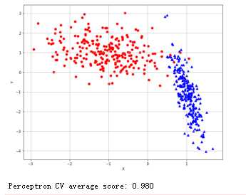
随机梯度下降法:
 1 from __future__ import print_function
 2
 3 import numpy as np
 4 import matplotlib.pyplot as plt
 5
 6 from sklearn.datasets import make_classification
 7 from sklearn.linear_model import SGDClassifier
 8 from sklearn.model_selection import cross_val_score
 9
10
11 # For reproducibility
12 np.random.seed(1000)
13
14 nb_samples = 500
15
16 def show_dataset(X, Y):
17     fig, ax = plt.subplots(1, 1, figsize=(10, 8))
18
19     ax.grid()
20     ax.set_xlabel(‘X‘)
21     ax.set_ylabel(‘Y‘)
22
23     for i in range(nb_samples):
24         if Y[i] == 0:
25             ax.scatter(X[i, 0], X[i, 1], marker=‘o‘, color=‘r‘)
26         else:
27             ax.scatter(X[i, 0], X[i, 1], marker=‘^‘, color=‘b‘)
28
29     plt.show()
30
31
32 if __name__ == ‘__main__‘:
33     # Create dataset
34     X, Y = make_classification(n_samples=nb_samples, n_features=2, n_informative=2, n_redundant=0,
35                                n_clusters_per_class=1)
36
37     # Show dataset
38     show_dataset(X, Y)
39
40     # Create perceptron as SGD instance
41     # The same result can be obtained using directly the class sklearn.linear_model.Perceptron
42     sgd = SGDClassifier(loss=‘perceptron‘, learning_rate=‘optimal‘, n_iter=10)
43     sgd_scores = cross_val_score(sgd, X, Y, scoring=‘accuracy‘, cv=10)
44     print(‘Perceptron CV average score: %.3f‘ % sgd_scores.mean())
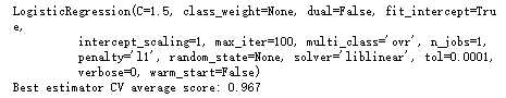
网格搜索找到最优超参数:
 1 from __future__ import print_function
 2 import numpy as np
 3 import multiprocessing
 4 from sklearn.datasets import load_iris
 5 from sklearn.model_selection import GridSearchCV, cross_val_score
 6 from sklearn.linear_model import LogisticRegression
 7 # For reproducibility
 8 np.random.seed(1000)
 9 if __name__ == ‘__main__‘:
10     # Load dataset
11     iris = load_iris()
12
13     # Define a param grid
14     param_grid = [
15         {
16             ‘penalty‘: [‘l1‘, ‘l2‘],
17             ‘C‘: [0.5, 1.0, 1.5, 1.8, 2.0, 2.5]
18         }
19     ]
20     # Create and train a grid search
21     gs = GridSearchCV(estimator=LogisticRegression(), param_grid=param_grid,
22                       scoring=‘accuracy‘, cv=10, n_jobs=multiprocessing.cpu_count())
23     gs.fit(iris.data, iris.target)
24     # Best estimator
25     print(gs.best_estimator_)
26     gs_scores = cross_val_score(gs.best_estimator_, iris.data, iris.target, scoring=‘accuracy‘, cv=10)
27     print(‘Best estimator CV average score: %.3f‘ % gs_scores.mean())
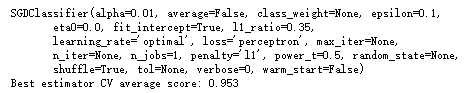
 1 from __future__ import print_function
 2 import numpy as np
 3 import multiprocessing
 4 from sklearn.datasets import load_iris
 5 from sklearn.model_selection import GridSearchCV, cross_val_score
 6 from sklearn.linear_model import SGDClassifier
 7 # For reproducibility
 8 np.random.seed(1000)
 9 if __name__ == ‘__main__‘:
10     # Load dataset
11     iris = load_iris()
12
13     # Define a param grid
14     param_grid = [
15         {
16             ‘penalty‘: [‘l1‘, ‘l2‘, ‘elasticnet‘],
17             ‘alpha‘: [1e-5, 1e-4, 5e-4, 1e-3, 2.3e-3, 5e-3, 1e-2],
18             ‘l1_ratio‘: [0.01, 0.05, 0.1, 0.15, 0.25, 0.35, 0.5, 0.75, 0.8]
19         }
20     ]
21     # Create SGD classifier
22     sgd = SGDClassifier(loss=‘perceptron‘, learning_rate=‘optimal‘)
23     # Create and train a grid search
24     gs = GridSearchCV(estimator=sgd, param_grid=param_grid, scoring=‘accuracy‘, cv=10,
25                       n_jobs=multiprocessing.cpu_count())
26     gs.fit(iris.data, iris.target)
27     # Best estimator
28     print(gs.best_estimator_)
29     gs_scores = cross_val_score(gs.best_estimator_, iris.data, iris.target, scoring=‘accuracy‘, cv=10)
30     print(‘Best estimator CV average score: %.3f‘ % gs_scores.mean())
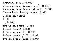
评估分类的指标:含混淆矩阵部分
 1 from __future__ import print_function
 2 import numpy as np
 3
 4 from sklearn.datasets import make_classification
 5 from sklearn.model_selection import train_test_split
 6 from sklearn.linear_model import LogisticRegression
 7 from sklearn.metrics import accuracy_score, zero_one_loss, jaccard_similarity_score, confusion_matrix,  8     precision_score, recall_score, fbeta_score
 9 # For reproducibility
10 np.random.seed(1000)
11 nb_samples = 500
12
13 if __name__ == ‘__main__‘:
14     # Create dataset
15     X, Y = make_classification(n_samples=nb_samples, n_features=2, n_informative=2, n_redundant=0,
16                                n_clusters_per_class=1)
17
18     # Split dataset
19     X_train, X_test, Y_train, Y_test = train_test_split(X, Y, test_size=0.25)
20     # Create and train logistic regressor
21     lr = LogisticRegression()
22     lr.fit(X_train, Y_train)
23     print(‘Accuracy score: %.3f‘ % accuracy_score(Y_test, lr.predict(X_test)))
24     print(‘Zero-one loss (normalized): %.3f‘ % zero_one_loss(Y_test, lr.predict(X_test)))
25     print(‘Zero-one loss (unnormalized): %.3f‘ % zero_one_loss(Y_test, lr.predict(X_test), normalize=False))
26     print(‘Jaccard similarity score: %.3f‘ % jaccard_similarity_score(Y_test, lr.predict(X_test)))
27     # Compute confusion matrix
28     cm = confusion_matrix(y_true=Y_test, y_pred=lr.predict(X_test))
29     print(‘Confusion matrix:‘)
30     print(cm)
31     print(‘Precision score: %.3f‘ % precision_score(Y_test, lr.predict(X_test)))
32     print(‘Recall score: %.3f‘ % recall_score(Y_test, lr.predict(X_test)))
33     print(‘F-Beta score (1): %.3f‘ % fbeta_score(Y_test, lr.predict(X_test), beta=1))
34     print(‘F-Beta score (0.75): %.3f‘ % fbeta_score(Y_test, lr.predict(X_test), beta=0.75))
35     print(‘F-Beta score (1.25): %.3f‘ % fbeta_score(Y_test, lr.predict(X_test), beta=1.25))
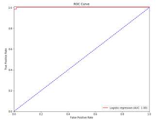
ROC曲线:
 1 from __future__ import print_function
 2
 3 import numpy as np
 4 import matplotlib.pyplot as plt
 5
 6 from sklearn.datasets import make_classification
 7 from sklearn.model_selection import train_test_split
 8 from sklearn.linear_model import LogisticRegression
 9 from sklearn.metrics import roc_curve, auc
10
11
12 # For reproducibility
13 np.random.seed(1000)
14
15 nb_samples = 500
16
17
18 if __name__ == ‘__main__‘:
19     # Create dataset
20     X, Y = make_classification(n_samples=nb_samples, n_features=2, n_informative=2, n_redundant=0,
21                                n_clusters_per_class=1)
22
23     # Split dataset
24     X_train, X_test, Y_train, Y_test = train_test_split(X, Y, test_size=0.25)
25
26     #Create and train logistic regressor
27     lr = LogisticRegression()
28     lr.fit(X_train, Y_train)
29
30     # Compute ROC curve
31     Y_score = lr.decision_function(X_test)
32     fpr, tpr, thresholds = roc_curve(Y_test, Y_score)
33
34     plt.figure(figsize=(10, 8))
35
36     plt.plot(fpr, tpr, color=‘red‘, label=‘Logistic regression (AUC: %.2f)‘ % auc(fpr, tpr))
37     plt.plot([0, 1], [0, 1], color=‘blue‘, linestyle=‘--‘)
38     plt.xlim([0.0, 1.0])
39     plt.ylim([0.0, 1.01])
40     plt.title(‘ROC Curve‘)
41     plt.xlabel(‘False Positive Rate‘)
42     plt.ylabel(‘True Positive Rate‘)
43     plt.legend(loc="lower right")
44
45     plt.show()
原文:https://www.cnblogs.com/bai2018/p/10581410.html
