from sklearn.datasets import fetch_mldata
from scipy.io import loadmat

mnist = fetch_mldata('MNIST original', transpose_data=True, data_home='files')
print(mnist)
# *DESCR为description,即数据集的描述
# *CLO_NAMES为列名
# *target键,带有标记的数组
# *data键,每个实例为一行,每个特征为1列
# 共七万张图片,每张图片784个特征点
X, y = mnist["data"], mnist["target"]
print(X.shape, y.shape)
# 显示图片
import matplotlib
import matplotlib.pyplot as plt

some_digit = X[36000]
some_digit_image = some_digit.reshape(28, 28)  # 将一维数组转化为28*28的数组
{'DESCR': 'mldata.org dataset: mnist-original', 'COL_NAMES': ['label', 'data'], 'target': array([0., 0., 0., ..., 9., 9., 9.]), 'data': array([[0, 0, 0, ..., 0, 0, 0],
[0, 0, 0, ..., 0, 0, 0],
[0, 0, 0, ..., 0, 0, 0],
...,
[0, 0, 0, ..., 0, 0, 0],
[0, 0, 0, ..., 0, 0, 0],
[0, 0, 0, ..., 0, 0, 0]], dtype=uint8)}
(70000, 784) (70000,)cmap->颜色图谱(colormap)
interpolation: 图像插值参数,图像插值就是利用已知邻近像素点的灰度值(或rgb图像中的三色值)来产生未知像素点的灰度值,以便由原始图像再生出具有更高分辨率的图像。
plt.imshow(some_digit_image, cmap=matplotlib.cm.binary,interpolation="nearest")
plt.axis("off")
plt.show()
print(y[36000])

# 批量查看数据样例
def plot_digits(instances, images_per_row=10, **options):
    size = 28
    images_per_row = min(len(instances), images_per_row)
    images = [instance.reshape(size,size) for instance in instances]
    n_rows = (len(instances) - 1) // images_per_row + 1
    row_images = []
    n_empty = n_rows * images_per_row - len(instances)
    images.append(np.zeros((size, size * n_empty)))
    for row in range(n_rows):
        rimages = images[row * images_per_row : (row + 1) * images_per_row]
        row_images.append(np.concatenate(rimages, axis=1))
    image = np.concatenate(row_images, axis=0)
    plt.imshow(image, cmap = matplotlib.cm.binary, **options)
    plt.axis("off")

import numpy as np
plt.figure(figsize=(9,9))
example_images = np.r_[X[:12000:600], X[13000:30600:600], X[30600:60000:590]]
plot_digits(example_images, images_per_row=10)
plt.show()
5.0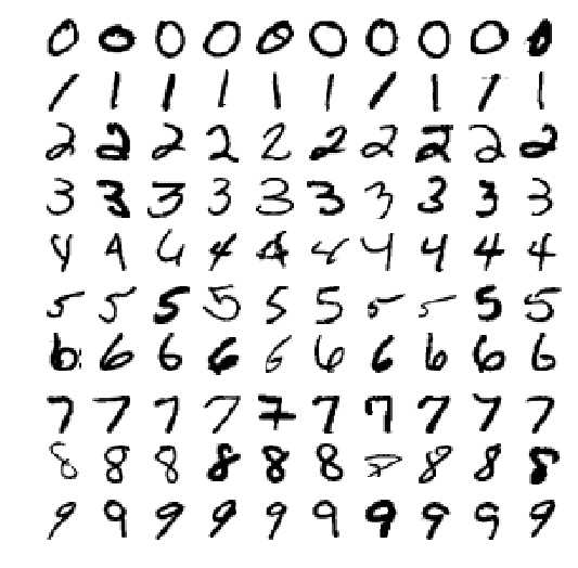
x_train, x_test, y_train, y_test = X[:60000], X[60000:], y[:60000], y[60000:]

import numpy as np
# Randomly permute a sequence, or return a permuted range.
shuffle_index = np.random.permutation(60000)
x_train, y_train = x_train[shuffle_index], y_train[shuffle_index]from sklearn.linear_model import SGDClassifier
y_train_5 = (y_train == 5) # True for all 5s, False for all other digits.
y_test_5 = (y_test == 5)sgd_clf = SGDClassifier(random_state=42)
sgd_clf.fit(x_train,y_train_5)
result = sgd_clf.predict([some_digit])
print(result)D:\Anaconda3\lib\site-packages\sklearn\linear_model\stochastic_gradient.py:144: FutureWarning: max_iter and tol parameters have been added in SGDClassifier in 0.19. If both are left unset, they default to max_iter=5 and tol=None. If tol is not None, max_iter defaults to max_iter=1000. From 0.21, default max_iter will be 1000, and default tol will be 1e-3.
FutureWarning)
[False]from sklearn.model_selection import StratifiedKFold
from sklearn.base import clone
skfolds = StratifiedKFold(n_splits=3,random_state=42)for train_index,test_index in skfolds.split(x_train,y_train_5):
clone_clf = clone(sgd_clf)
x_train_folds = x_train[train_index]
y_train_folds = (y_train_5[train_index])
x_test_fold = x_train[test_index]
y_test_fold = (y_train_5[test_index])
clone_clf.fit(x_train_folds,y_train_folds)
y_pred = clone_clf.predict(x_test_fold) # 将所有预测正确的结果加起来
n_correct = sum(y_pred == y_test_fold)
print(n_correct/len(y_pred))0.9455
0.9636
0.95855from sklearn.model_selection import cross_val_score
array = cross_val_score(sgd_clf,x_train,y_train_5,cv=3,scoring="accuracy")
print(array)[0.9455 0.9636 0.95855]from sklearn.base import BaseEstimator
class Never5Clissifer(BaseEstimator):
def fit (self,x,y=None):
pass
def predict (self,x):
return np.zeros((len(x),1),dtype=bool)
never_5_clf = Never5Clissifer()
array = cross_val_score(never_5_clf,x_train,y_train_5,cv=3,scoring="accuracy")
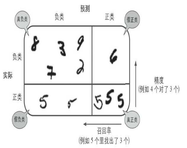
print(array)[0.9078 0.9121 0.90905]所谓混淆矩阵,就是指类别与类别之间分类错误的次数。 例如,数字3被错误分成数字5的次数会
记录在第5行第三列。这里使用corss_val_predict来预测,返回的指是每个折叠的预测。cross_val_predict()
通过K-fold折叠返回3组预测值,这3组测试的数据是相互隔离的,每一次预测的数据在训练期间是没见过的。
混淆矩阵中,行表示实际类别,列表示预测类别。如:
\begin{matrix}
x & y \
z & v
\end{matrix}
第0行0列表示非6的图片(负类)分类成了非6的数量(成为真负类数量);
第0行第1列表示非6的图片分类成了6的的数量(假正类);
第1行第0列表示是6的图片(正类)分类成了非6的数量(假负类);
第1行第1列表示是6的图片分类成了6的数量(真正类)。
所以在完美情况下,混淆矩阵只有对角线有非零值,其余均为0
混淆矩阵图示:
from sklearn.model_selection import cross_val_predict
y_train_pred = cross_val_predict(sgd_clf,x_train,y_train_5,cv=3)
from sklearn.metrics import confusion_matrix
array= confusion_matrix(y_train_5,y_train_pred)
array_perfect = confusion_matrix(y_train_5,y_train_5)
print(array)
print("perfect:",array_perfect)
[[53537 1042]
[ 1605 3816]]
perfect: [[54579 0]
[ 0 5421]]1.利用混淆矩阵计算分类器的精度。$$精度 = \frac{TP}{TP+FP} (TP->真正类,FP->假正类)$$
精确率是针对我们预测结果而言的,它表示的是预测为正的样本中有多少是真正的正样本。
2.利用混淆矩阵计算召回率(recall),也叫做灵敏度(ensitivity)或者真正类率(TPR)。$$召回率=\frac{TP}{TP+FN} (FN->假负类)$$
召回率是针对我们原来的样本而言的,它表示的是样本中的正例有多少被预测正确了。
3.$F_1$分数,是精度和召回率的组合(谐波平均值,对于较低的值更高的权重,而不是传统的一视同仁)。
所以只有当召回率和精度都很高的时候,分类器的$F_1$分数才会比较高。
$$F_1 = \frac{2}{\frac{1}{精度}+{\frac{1}{召回率}}} = 2 \times \frac{精度\times召回率}{精度+召回率} = \frac{TP}{TP+\frac{FN+FP}{2}} $$
from sklearn.metrics import precision_score,recall_score
print(precision_score(y_train_5,y_train_pred))
print(recall_score(y_train_5,y_train_pred))
from sklearn.metrics import f1_score
print(f1_score(y_train_5,y_train_pred))
0.785508439687114
0.703929164360819
0.742484677497811y_scores = sgd_clf.decision_function([some_digit])
print(y_scores)
threshold = 0
y_some_digit_pred = (y_scores>threshold)
print("threshold=0",y_some_digit_pred) # 当阈值比较小的时候为True
threshold = 600000 # 提升阈值
y_some_digit_pred = (y_scores>threshold)
print("threshold=600000",y_some_digit_pred) # 当阈值比较大的时候为False[-19662.17519015]
threshold=0 [False]
threshold=600000 [False]上面两个结果的变化说明,阈值的变化会改变召回率。那么如何达到准确率和召回率的平衡呢(选取最好的阈值)?
y_scores = cross_val_predict(sgd_clf,x_train,y_train_5,cv=3,method="decision_function")
from sklearn.metrics import precision_recall_curve
precisions,recalls,thresholds = precision_recall_curve(y_train_5,y_scores)
def plot_precision_recall_vs_threshold(precisions,recalls,thresholds):
    plt.plot(thresholds,precisions[:-1],"r--",label="Precision") # 绘图(x,y,表示符号,标签)
    plt.plot(thresholds,recalls[:-1],"g--",label ="Recall")
    plt.xlabel("Threshold")
    plt.legend(loc="upper left") # 图例的位置
    plt.ylim([0,1])
plot_precision_recall_vs_threshold(precisions,recalls,thresholds)
plt.show()

# 指定精度/召回率的分类器
y_train_pred_90 = (y_scores>700000) # 阈值从图上找
print(precision_score(y_train_5,y_train_pred_90))
print(recall_score(y_train_5,y_train_pred_90))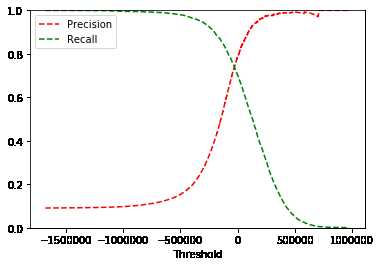
0.9714285714285714
0.006271905552481092from sklearn.metrics import roc_curve
fpr,tpr,thresholds = roc_curve(y_train_5,y_scores)
def plot_roc_curve(fpr,tpr,label=None):
plt.plot(fpr,tpr,lineWidth=2,label=label)
plt.plot([0,1],[0,1],"k--")
plt.axis([0,1,0,1]) # 设置x轴,y轴的起始和终点
plt.xlabel('False Positive Rate')
plt.ylabel('True Positive Rate')
plot_roc_curve(fpr,tpr)
plt.show()
from sklearn.metrics import roc_auc_score
print(roc_auc_score(y_train_5,y_scores))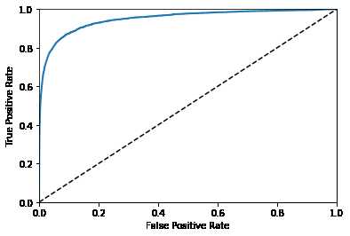
0.950155100287553绘制RF分类器的ROC曲线:
from sklearn.ensemble import RandomForestClassifier
rf_clf = RandomForestClassifier(random_state=42)
y_rf_clf = cross_val_predict(rf_clf,x_train,y_train_5,cv=3,method="predict_proba")
print(y_rf_clf)

y_scores_rf = y_rf_clf[:,1]  # 分数为正样本的概率,即取二维数组每一行的第二个数据
fpr_rf,tpr_rf,thresholds_rf = roc_curve(y_train_5,y_scores_rf)
plt.plot(fpr,tpr,"b:",label="SGD")
plot_roc_curve(fpr_rf,tpr_rf,"Random Forest")
plt.legend(loc="lower right")
plt.show()
print(roc_auc_score(y_train_5,y_scores_rf))
[[1. 0. ]
[0.9 0.1]
[0.9 0.1]
...
[1. 0. ]
[1. 0. ]
[1. 0. ]]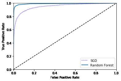
0.9917598412633858多分类策略(以MNIST为例):
sgd_clf.fit(x_train,y_train)
array = sgd_clf.predict([some_digit])
print(array)   # array([5.])
some_digit_score = sgd_clf.decision_function([some_digit])
print(some_digit_score)
# 上面代码中,sgd训练时训练了所有0-9的数据(OVA),在内部生成了10个分类器,some_digit_score就是十个分类器的分数。在预测时,取了最高的分数给出结果
from sklearn.multiclass import OneVsOneClassifier
ovo_clf = OneVsOneClassifier(SGDClassifier(random_state=42))
ovo_clf.fit(x_train,y_train)
array = ovo_clf.predict([some_digit])
print("result:",array)                                              #结果
print("length of ovo_clf",len(ovo_clf.estimators_))                 #分类器个数
# RF的多分类策略(RD可以直接将实例分为多个类别)
rf_clf.fit(x_train,y_train)
rf_clf.predict([some_digit])
print("RF的各个类概率:",rf_clf.predict_proba([some_digit]))          #RF中各个类的概率
[5.]
[[-193260.69253369 -268272.35422435 -160594.339744 -157709.0339379
-532207.50918753 -19662.17519015 -781920.88031095 -280417.97366431
-856441.40614529 -552502.53905182]]
result: [5.]
length of ovo_clf 45
RF的各个类概率: [[0.1 0. 0. 0.1 0. 0.8 0. 0. 0. 0. ]]array = cross_val_score(sgd_clf,x_train,y_train,cv=3,scoring="accuracy")
print("3折交叉检验:",array)
from sklearn.preprocessing import StandardScaler
scaler = StandardScaler()
x_train_scaler = scaler.fit_transform(x_train.astype(np.float64)) # astype:数据类型转换
array = cross_val_score(sgd_clf,x_train_scaler,y_train,cv=3,scoring="accuracy")
print("特征缩放后的准确率:",array)3折交叉检验: [0.85472905 0.86074304 0.86738011]
特征缩放后的准确率: [0.90826835 0.90894545 0.91053658]# 生成混淆矩阵
y_train_pred = cross_val_predict(sgd_clf,x_train_scaler,y_train,cv=3)
conf_mx = confusion_matrix(y_train,y_train_pred)
print(conf_mx)
plt.matshow(conf_mx,cmap=plt.cm.gray)
plt.show()[[5733 2 22 8 9 50 47 7 42 3]
[ 2 6490 44 25 6 41 8 13 100 13]
[ 59 37 5319 97 83 26 99 62 159 17]
[ 43 42 128 5345 1 232 32 53 142 113]
[ 20 25 39 8 5385 9 49 32 73 202]
[ 70 38 32 212 80 4574 112 27 173 103]
[ 36 25 44 2 39 104 5624 4 40 0]
[ 25 21 62 24 64 12 4 5793 12 248]
[ 52 156 67 145 17 158 50 26 5023 157]
[ 44 33 24 80 172 38 2 210 77 5269]]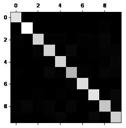
# 计算每个类别的错误率
row_sums = conf_mx.sum(axis=1, keepdims=True)  # keepdims用来保持矩阵的多维特征,也就是sum操作后还是跟混淆矩阵一样的二维矩阵)
norm_conf_mx = conf_mx / row_sums

# 用0填充对角线,只保留错误。
np.fill_diagonal(norm_conf_mx,0)               # 填充任意维度矩阵的主对角线
plt.matshow(norm_conf_mx,cmap=plt.cm.gray)
plt.show()
# 结果分析:每一行代表实际类别,每一列代表被分类的类别。越暗说明越正确。比如第4行的第9列很亮,表示
# 有很多的4被错误分成了9. 同样,有不少8被错误分为了1、3、5、9等数字。混淆矩阵可以直观的看出来每个
# 分类的具体情况。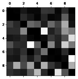
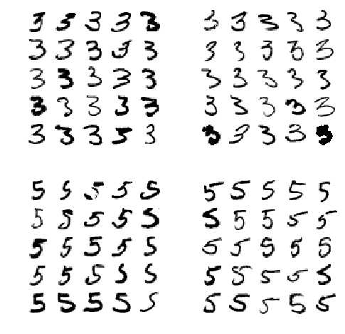
# 组合显示样例图片
cl_a, cl_b = 3, 5
x_aa = x_train[(y_train == cl_a) & (y_train_pred == cl_a)]
x_ab = x_train[(y_train == cl_a) & (y_train_pred == cl_b)]
x_ba = x_train[(y_train == cl_b) & (y_train_pred == cl_a)]
x_bb = x_train[(y_train == cl_b) & (y_train_pred == cl_b)]

plt.figure(figsize=(8, 8))
plt.subplot(221)                                # subplot:组合很多小图,放到大图里面显示
plot_digits(x_aa[:25], images_per_row=5)
plt.subplot(222)
plot_digits(x_ab[:25], images_per_row=5)
plt.subplot(223)
plot_digits(x_ba[:25], images_per_row=5)
plt.subplot(224)
plot_digits(x_bb[:25], images_per_row=5)
plt.show()
from sklearn.neighbors import KNeighborsClassifier
y_train_large = (y_train>=7)                      # 标签1:数字是否大于等于7
y_train_odd = (y_train%2==1)                      # 标签2:数字是否为奇数
y_multilabel = np.c_[y_train_large,y_train_odd]

knn_clf = KNeighborsClassifier()                  # 训练一个KNN分类器
knn_clf.fit(x_train,y_multilabel)
array = knn_clf.predict([some_digit])
print(array)
[[False True]]y_train_knn_pred = cross_val_predict(knn_clf,x_train,y_train,cv=3)
f1_score(y_train,y_train_knn_pred,average="macro")
noise = np.random.randint(0, 100, (len(x_train), 784))      # 给图片加噪声
X_train_mod = x_train + noise
noise = np.random.randint(0, 100, (len(x_test), 784))
X_test_mod = x_test + noise
y_train_mod = x_train
y_test_mod = x_test
some_index = 5500
plt.subplot(121); plot_digits(X_test_mod[some_index])
plt.subplot(122); plot_digits(y_test_mod[some_index])
plt.show()

knn_clf.fit(X_train_mod, y_train_mod)
clean_digit = knn_clf.predict([X_test_mod[some_index]])
plot_digits(clean_digit)
Hand on Machine Learning 第三章:分类器
原文:https://www.cnblogs.com/NewBee-CHH/p/10880933.html