use gradient descent to achieve liner regression (Matlab)

# what‘s the Supervised learning

Always we want to use the data we have to predict the part we don‘t know. And we prefer to find a mathematical function to predict. Therefore Supervised learning was created.

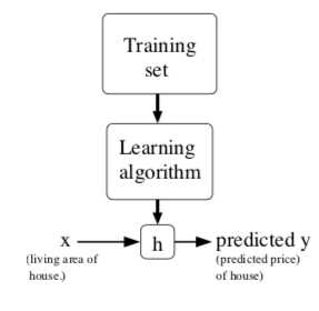
As we said above, "Training set" is the data we have, and the "learning algorithm" is a strategy to help us get the mathematical function. the lower case "h" means "hypothesis"(for some historical reasons) and that‘s the mathematical function to predict.

Let‘s give a definition more formally, Supervised learning: "given a training set, to learn a function h: X -> Y so that h(x) is a "good" predictor for the corresponding value of y."

# regression problem and classification problem

we still focus on the structure chart above, the difference between a regression problem and a classification problem is "dose the predicted y is continuous".

if we are trying to predict is continuous, we call the learning problem is a regression problem. When y can take on only a small number of discrete values, we call it a classification problem.

# Linear Regression 

Let‘s start with a simple example. we get a set of training examples -- "three points (1,1) (2,2) (3,2)". and we want to get a line helping us to predict. We easily know that these points cannot in the same line. so how we can get a "good" predictor?

First of all, let‘s say we decide to approximate y as a linear function of x: h_Θ(x) = Θ₀+Θ₁x.

Here, the Θ_i‘s are the parameters (also called weights) parameterizing the space of liner functions mapping from X to Y.

Now, given a training set, how do we pick, or learn the parameters Θ?

One reasonable way is to make h(x) close to y. To formalize this, we define a function(cost function):

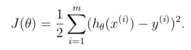
// notation:  m: the number of training example

//x = "input" variables/features

//y = "out" variables/targets

//(xⁱ,yⁱ): the ith traning example 

# gradient descent

Now our problem is changed to minimize J(Θ).

before that let‘s consider the gradient descent algorithm:

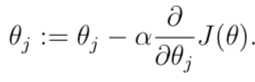
 // It starts with some initial Θ and repeatedly performs the update.

//as for why we can get the minimum Θ, it‘s about a piece of mathematical knowledge.

now we do some simplifying.

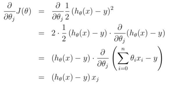
therefore, we get the following algorithm:

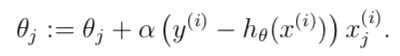// For a single training example.

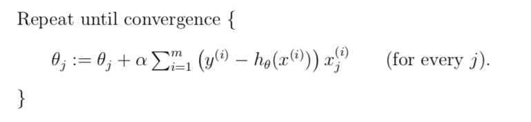//batch gradient descent

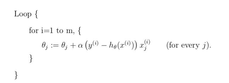//stochastic gradient descent

 and the following code is using Matlab to solve the simple problem above.

clear all
clc

% hypothesis
theta0 = 1;
theta1 = 1;
x = [1;2;3];
y = [1;2;2];

% gradient descent
alpha = 0.01;
for k = 1:5000
    time = k;
    hypothesis = theta0 + theta1*x;
    %cost function
    %cost = sum((hypothesis - y).^2)/3;
    r0 = sum(hypothesis - y);
    theta0 = theta0 - alpha*r0;
    r1 = sum((hypothesis - y).*x);
    theta1 = theta1 - alpha*r1;
end

use gradient descent to achieve liner regression (Matlab)

原文：https://www.cnblogs.com/Samuel514/p/11420298.html