#三大件
import numpy as np
import pandas as pd
import matplotlib.pyplot as plt
%matplotlib inline
我们将建立一个逻辑回归模型来预测一个学生是否被大学录取。
假设你是一个大学系的管理员,你想根据两次考试的结果来决定每个申请人的录取机会。
你有以前的申请人的历史数据,你可以用它作为逻辑回归的训练集。
对于每一个培训例子,你有两个考试的申请人的分数和录取决定。
为了做到这一点,我们将建立一个分类模型,根据考试成绩估计入学概率。
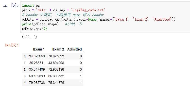
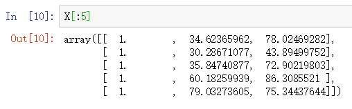
import os
path = ‘data‘ + os.sep + ‘LogiReg_data.txt‘
pdData = pd.read_csv(path, header=None, names=[‘Exam 1‘, ‘Exam 2‘, ‘Admitted‘])
pdData.head()
pdData.shape   #(100, 3) 数据维度 100 行, 3列
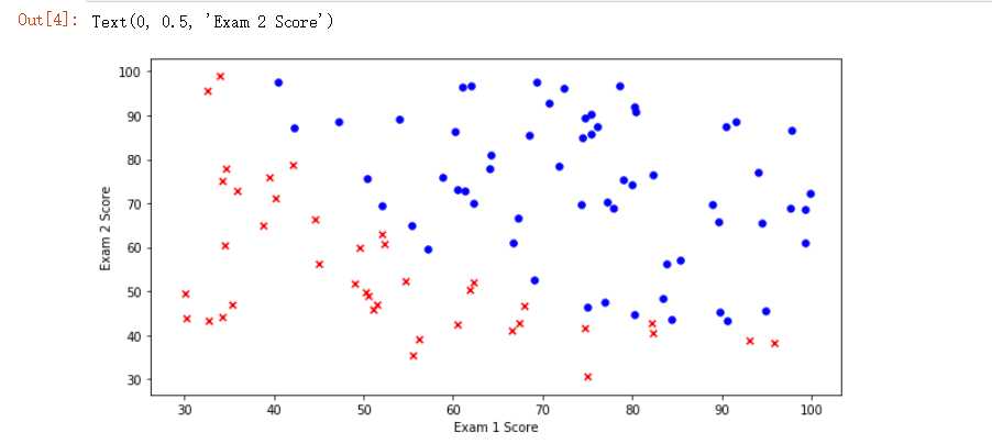
positive = pdData[pdData[‘Admitted‘] == 1] # returns the subset of rows such Admitted = 1, i.e. the set of *positive* examples
negative = pdData[pdData[‘Admitted‘] == 0] # returns the subset of rows such Admitted = 0, i.e. the set of *negative* examples

fig, ax = plt.subplots(figsize=(10,5))
ax.scatter(positive[‘Exam 1‘], positive[‘Exam 2‘], s=30, c=‘b‘, marker=‘o‘, label=‘Admitted‘)
ax.scatter(negative[‘Exam 1‘], negative[‘Exam 2‘], s=30, c=‘r‘, marker=‘x‘, label=‘Not Admitted‘)
ax.legend() # 展示图形标识
ax.set_xlabel(‘Exam 1 Score‘) # x 标识
ax.set_ylabel(‘Exam 2 Score‘) # y 标识
? 建立分类器
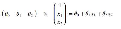
? 求解三个参数  - 分别表示 成绩一, 成绩二以及偏置项的参数
? 设定阈值来标识分类的结果, 此处设置为 0.5
? > 0.5 标识通过, < 0.5 标识未通过
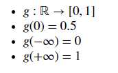
? sigmoid : 映射到概率的函数
? model : 返回预测结果值
? cost : 根据参数计算损失
? gradient : 计算每个参数的梯度方向
? descent : 进行参数更新
? accuracy: 计算精度
sigmoid 函数实现 ? 公式 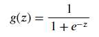
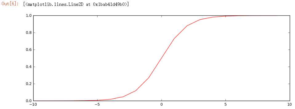
? Python 实现 def sigmoid(z): return 1 / (1 + np.exp(-z))
? 画图展示
nums = np.arange(-10, 10, step=1) #creates a vector containing 20 equally spaced values from -10 to 10
fig, ax = plt.subplots(figsize=(12,4))
ax.plot(nums, sigmoid(nums), ‘r‘)
? 值域
? 数学公式 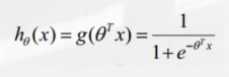
? Python 实现
def model(X, theta):

    return sigmoid(np.dot(X, theta.T))
? 加一行 - 数据集要进行偏置项的处理 ( 加一列全1的数据 )
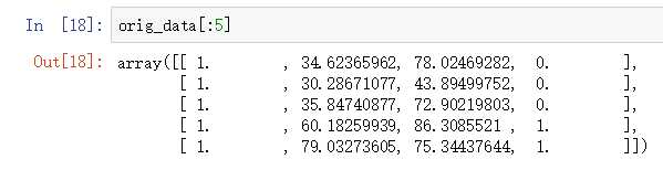
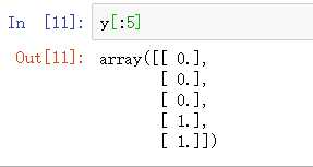
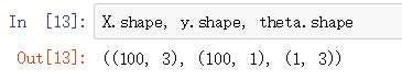
pdData.insert(0, ‘Ones‘, 1) # 偏置项参数的处理


# set X (training data/训练数据) and y (target variable/变量参数)
orig_data = pdData.as_matrix() # 转换为 数组形式
cols = orig_data.shape[1]
X = orig_data[:,0:cols-1]
y = orig_data[:,cols-1:cols]

# convert to numpy arrays and initalize the parameter array theta
#X = np.matrix(X.values)
#y = np.matrix(data.iloc[:,3:4].values) #np.array(y.values)
theta = np.zeros([1, 3])  # 参数占位, 先用 0 填充
? 数学公式
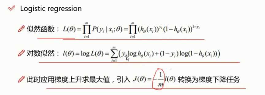
将对数似然函数去负号 - ![]()
求平均损失 - 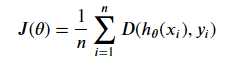
这块如果忘了怎么回事可以在这里进行查阅 点击这里跳转公式篇
? Python 实现
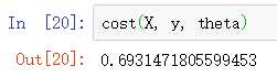
def cost(X, y, theta):
    left = np.multiply(-y, np.log(model(X, theta)))
    right = np.multiply(1 - y, np.log(1 - model(X, theta)))
    return np.sum(left - right) / (len(X))
X, y 表示两个特征值, 传入 theta 表示参数 
np.multiply 乘法计算, 将式子分为左右查分
? 计算 cost 值
? 数学公式 - 进行求导计算后, 将最终结果转换为 python 实现
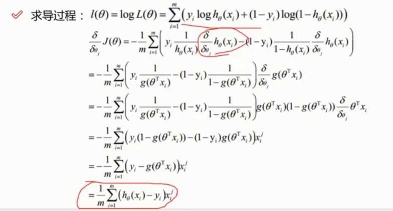
![]()
? Python 实现
def gradient(X, y, theta):
    grad = np.zeros(theta.shape) # 因为会有三个结果, 因此这里进行预先的占位
    error = (model(X, theta)- y).ravel() # h0(xi)-yi 象形... 这里吧前面的m分之一的那个负号移到了这里来去除负号
    for j in range(len(theta.ravel())): # 求三次
        term = np.multiply(error, X[:,j]) # : 表示所有的行, j 表示第 j 列
        grad[0, j] = np.sum(term) / len(X)

    return grad
这里有三个 , 那么应该也是计算出来三个值, 因此这里进行了三次的循环
每次的循环针对要处理的那一列进行操作
STOP_ITER = 0 # 根据迭代次数, 达到迭代次数及停止
STOP_COST = 1 # 根据损失, 损失差异较小及停止
STOP_GRAD = 2 # 根据梯度, 梯度变化较小则停止

def stopCriterion(type, value, threshold):
    #设定三种不同的停止策略
    if type == STOP_ITER:        return value > threshold
    elif type == STOP_COST:      return abs(value[-1]-value[-2]) < threshold
    elif type == STOP_GRAD:      return np.linalg.norm(value) < threshold
import numpy.random
#洗牌
def shuffleData(data):
    np.random.shuffle(data)
    cols = data.shape[1]
    X = data[:, 0:cols-1]
    y = data[:, cols-1:]
    return X, y
初始的数据集很大可能性是有做过排序的, 因此需要进行洗牌
然后重新生成我们需要的数据
import time

def descent(data, theta, batchSize, stopType, thresh, alpha):
    #梯度下降求解

    init_time = time.time()
    i = 0 # 迭代次数
    k = 0 # batch
    X, y = shuffleData(data)
    grad = np.zeros(theta.shape) # 计算的梯度
    costs = [cost(X, y, theta)] # 损失值


    while True:
        grad = gradient(X[k:k+batchSize], y[k:k+batchSize], theta)
        k += batchSize #取batch数量个数据
        if k >= n:
            k = 0
            X, y = shuffleData(data) #重新洗牌
        theta = theta - alpha*grad # 参数更新
        costs.append(cost(X, y, theta)) # 计算新的损失
        i += 1

        if stopType == STOP_ITER:       value = i
        elif stopType == STOP_COST:     value = costs
        elif stopType == STOP_GRAD:     value = grad
        if stopCriterion(stopType, value, thresh): break

    return theta, i-1, costs, grad, time.time() - init_time
? 参数详解
def runExpe(data, theta, batchSize, stopType, thresh, alpha):
    #import pdb; pdb.set_trace();
    theta, iter, costs, grad, dur = descent(data, theta, batchSize, stopType, thresh, alpha)  # 这是最核心的代码

    name = "Original" if (data[:,1]>2).sum() > 1 else "Scaled"
    name += " data - learning rate: {} - ".format(alpha)
    # 根据传入参数选择下降方式
    if batchSize==n: strDescType = "Gradient"  #  批量
    elif batchSize==1:  strDescType = "Stochastic"  # 随机
    else: strDescType = "Mini-batch ({})".format(batchSize) # 小批量
    name += strDescType + " descent - Stop: "
    # 根据 停止方式进行选择处理生成 name
    if stopType == STOP_ITER: strStop = "{} iterations".format(thresh)
    elif stopType == STOP_COST: strStop = "costs change < {}".format(thresh)
    else: strStop = "gradient norm < {}".format(thresh)
    name += strStop
    print ("***{}\nTheta: {} - Iter: {} - Last cost: {:03.2f} - Duration: {:03.2f}s".format(
        name, theta, iter, costs[-1], dur))
    # 画图
    fig, ax = plt.subplots(figsize=(12,4))
    ax.plot(np.arange(len(costs)), costs, ‘r‘)
    ax.set_xlabel(‘Iterations‘)
    ax.set_ylabel(‘Cost‘)
    ax.set_title(name.upper() + ‘ - Error vs. Iteration‘)
    return theta
此函数进行画图的一些名字的显示以及图形进行的简单的功能封装函数
可以理解为一个工具函数, 自动根据参数选择画图的某些调节比如标题等
n=100
runExpe(orig_data, theta, n, STOP_ITER, thresh=5000, alpha=0.000001)
? 参数详解
? 测试结果
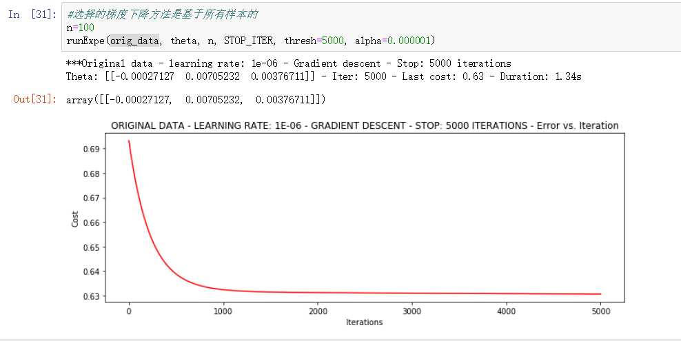
? 结果详解
1.34s 完成了全部的 5000次 迭代, 最终的结果的为 0.63 左右
runExpe(orig_data, theta, n, STOP_COST, thresh=0.000001, alpha=0.001)
? 参数详解
? 测试结果
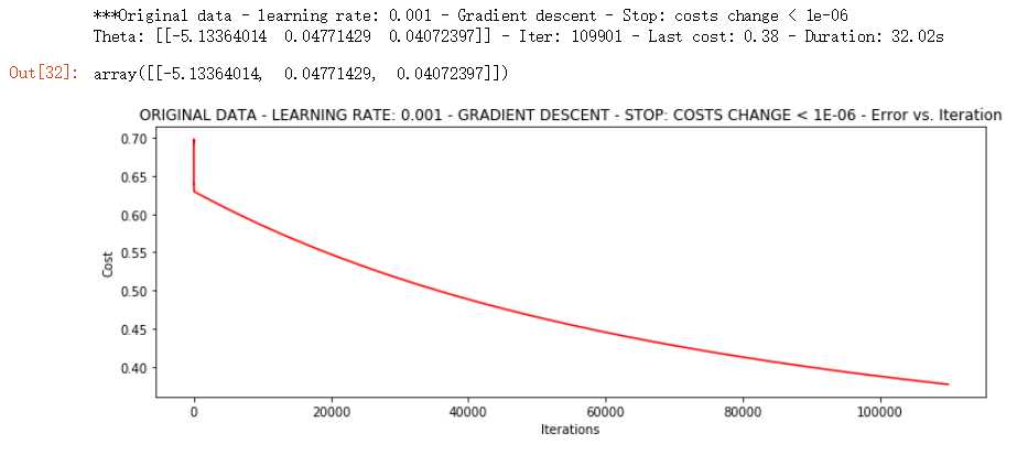
? 结果详解
可见测试用了 32.02s才完成, 达到损失值这么小的时候用了 100000次以上的迭代次数, 但是结果也达到了 0.4 以下
比上一轮的结果要优秀很多
runExpe(orig_data, theta, n, STOP_GRAD, thresh=0.05, alpha=0.001)
? 参数详解
? 测试结果
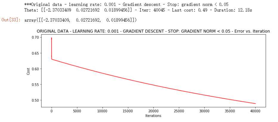
? 结果详解
可见测试用了12.18s 才完成, 达到损失值这么小的时候用了40000 次以上的迭代次数, 但是结果也达到了 0.5 以下
由迭代次数也可以看出比不过 12w 次的结果, 因此最终的收敛在 0.50 左右无法比过 0.4 的上轮结果
原文:https://www.cnblogs.com/shijieli/p/11431835.html