逻辑回归的假设函数为sigmoid函数,把较大范围变化的输出值挤压到(0,1)内,因此也被称为挤压函数
\[
h_\theta(x)=\frac{1}{1+e^{-\theta^Tx}}\tag{4.1}
\]
\(h_\theta(x)\)代表输入为x时y=1的概率
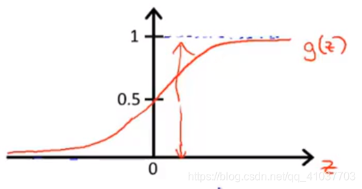
若规定\(h_\theta(x)\ge0.5\)时y=1,\(h_\theta(x)<0.5\)时y=0,则可得出当\(\theta^Tx\ge0\)时y=1,当\(\theta^Tx<0\)时y=0
若拟合确定参数\(\theta\)后,\(\theta^Tx\)构成决策边界
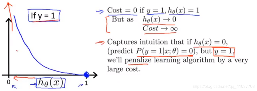
若用线性回归的代价函数,sigmoid函数会导致产生非凸函数,梯度下降法会陷入局部最优。
\[
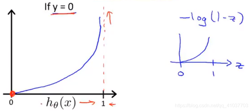
\text{Cost}(h_\theta(x),y)=\begin{cases}
-log(h_\theta(x)),&\text{if}\ y=1\-log(1-h_\theta(x)),&\text{if}\ y=0
\end{cases}\tag{4.2}
\]
\[ \begin{aligned} J(\theta) &=\frac{1}{m} \sum_{i=1}^{m} \operatorname{cost}(h_{\theta}(x^{(i)}), y^{(i)}) \\ &=-\frac{1}{m}[\sum_{i=1}^{m} y^{(i)} \log h_{\theta}(x^{(i)})+(1-y^{(i)}) \log (1-h_{\theta}(x^{(i)}))] \end{aligned}\tag{4.3} \]
再用不同算法使代价函数最小
\[ \begin{aligned} \theta_j&=\theta_j-\alpha\frac{\partial}{\partial\theta_j}J(\theta)\&=\theta_j-\alpha\sum_{i=1}^m(h_\theta(x^{(i)})-y^{(i)})x_j^{(i)} \end{aligned}\tag{4.4} \]
无需手动选择学习率,且收敛速度高于梯度下降法,但算法更为复杂
每次提取一个类别作为正类,其余为负类,重复多次得出多个假设函数作为多个分类器
对新样本预测时,分别使用每个分类器进行预测,并汇总所有结果,分类最多的结果作为对新样本的预测结果
原文:https://www.cnblogs.com/jestland/p/11548485.html