Self-Consistent Method (II)

Considering two dimensional cases, the distribution of electric potential can be obtained by solving Laplace’s and Poisson‘s Equation based on various boundary conditions.

(1) Laplace’s Equation

For a parallel-plate capacitor, the electric potential on the left and right is -1 and 1 respectively.

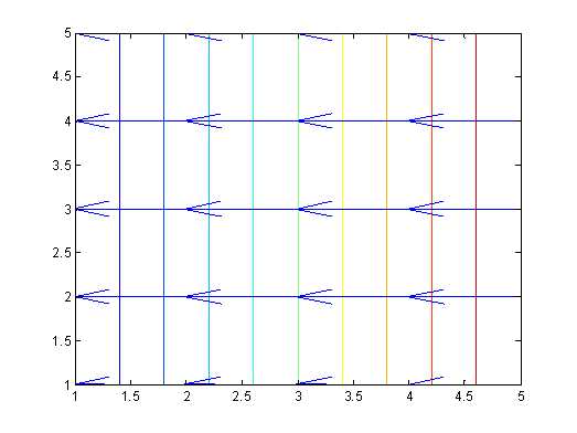
Here we divide the region into 5x5, where the  electric potential  is the matrix V. The first and last collumns are set to be -1 and 1.  The first and last rows are linspace(-1,1,N), which is the correct values for the boundary. Inside the region, V(i,j) can be obtained based on the fomular above (lines 8-12). We also use ‘while-end‘ loop to find the solution with given tolerence.

clear
N=5;
V=zeros(N,N);V(:,1)=-1;V(:,end)=1;V(1,:)=linspace(-1,1,N);
V(end,:)=linspace(-1,1,N);
dV=1;
while dV>0.0001
  V2=V;
for i=2:N-1
  for j=2:N-1
    V2(i,j)=0.25*(V(i+1,j)+V(i-1,j)+V(i,j+1)+V(i,j-1));
  endfor
endfor
dV=sum(sum(abs(V2-V)));
V=V2;
end

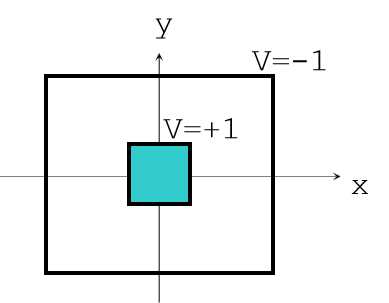
Another example is shown. The electric potential is 1 in the center (line 5). In the iteration (lines 8-12), the potential will be modified. Thus, we update it with the same initial distribution(line 14) .  

clear
N=11;
V=zeros(N,N);V(:,1)=-1;V(:,end)=-1;
V(1,:)=-1;V(end,:)=-1;
V((N+1)/2-2:(N+1)/2+2,(N+1)/2-2:(N+1)/2+2)=1;
dV=1;
while dV>0.0001
  V2=V;
for i=2:N-1
  for j=2:N-1
    V2(i,j)=0.25*(V(i+1,j)+V(i-1,j)+V(i,j+1)+V(i,j-1));
  endfor
endfor
V2((N+1)/2-2:(N+1)/2+2,(N+1)/2-2:(N+1)/2+2)=1;
dV=sum(sum(abs(V2-V)));
V=V2;
end

(2) Possibon Equation

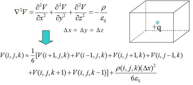
 When charges are concluded, the electronic potentials obeys Poisson EQ. We can introduce a matrix of chg (line 4), representing the charge distribution. The iteration of V(i,j) is also modified according to the equation (line 12).

clear
N=21;
V=zeros(N,N);
chg=V;chg(11,11)=1;
V(:,1)=-1;V(:,end)=-1;
V(1,:)=-1;V(end,:)=-1;
dV=1;
while dV>0.0001
  V2=V;
for i=2:N-1
  for j=2:N-1
    V2(i,j)=chg(i,j)+0.25*(V(i+1,j)+V(i-1,j)+V(i,j+1)+V(i,j-1));
  endfor
endfor
dV=sum(sum(abs(V2-V)));
V=V2;
end
　　

Self-Consistent Method (II)

原文：https://www.cnblogs.com/xbyang99/p/11757505.html