%matplotlib inline
import numpy as np
import matplotlib.pyplot as plt
from scipy import stats

import seaborn as sns;sns.set() # 使用seaborn的默认设置
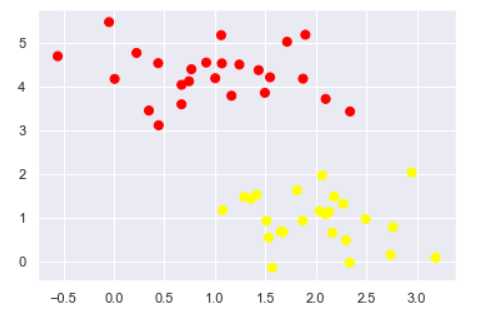
这里自己生成一些随机数据
#随机来点数据
from sklearn.datasets.samples_generator import make_blobs
X, y = make_blobs(
    n_samples=50, # 样本点数量
    centers=2,  # 簇堆数量
    random_state=0,  # 随机种子
    cluster_std=0.60  # 簇离散程度
)
plt.scatter(X[:, 0], X[:, 1], c=y, s=50, cmap=‘autumn‘)
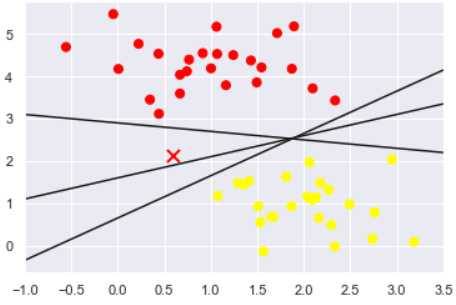
xfit = np.linspace(-1, 3.5)
plt.scatter(X[:, 0], X[:, 1], c=y, s=50, cmap=‘autumn‘)
plt.plot([0.6], [2.1], ‘x‘, color=‘red‘, markeredgewidth=2, markersize=10)

for m, b in [(1, 0.65), (0.5, 1.6), (-0.2, 2.9)]:
    plt.plot(xfit, m * xfit + b, ‘-k‘)

plt.xlim(-1, 3.5);
如图所示分开有很多种方式, 看哪种更好呢?
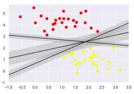
xfit = np.linspace(-1, 3.5)
plt.scatter(X[:, 0], X[:, 1], c=y, s=50, cmap=‘autumn‘)

for m, b, d in [(1, 0.65, 0.33), (0.5, 1.6, 0.55), (-0.2, 2.9, 0.2)]:
    yfit = m * xfit + b
    plt.plot(xfit, yfit, ‘-k‘)
    plt.fill_between(xfit, yfit - d, yfit + d, edgecolor=‘none‘,
                     color=‘#AAAAAA‘, alpha=0.4)

plt.xlim(-1, 3.5);
画出来他的决策边界即可看出宽度
from sklearn.svm import SVC # "Support vector classifier"
model = SVC(kernel=‘linear‘)
model.fit(X, y)
SVC(C=1.0, cache_size=200, class_weight=None, coef0=0.0,
  decision_function_shape=None, degree=3, gamma=‘auto‘, kernel=‘linear‘,
  max_iter=-1, probability=False, random_state=None, shrinking=True,
  tol=0.001, verbose=False)
#绘图函数
def plot_svc_decision_function(model, ax=None, plot_support=True):
    """Plot the decision function for a 2D SVC"""
    if ax is None:
        ax = plt.gca()
    xlim = ax.get_xlim()
    ylim = ax.get_ylim()

    # create grid to evaluate model
    x = np.linspace(xlim[0], xlim[1], 30)
    y = np.linspace(ylim[0], ylim[1], 30)
    Y, X = np.meshgrid(y, x)
    xy = np.vstack([X.ravel(), Y.ravel()]).T
    P = model.decision_function(xy).reshape(X.shape)

    # plot decision boundary and margins
    ax.contour(X, Y, P, colors=‘k‘,
               levels=[-1, 0, 1], alpha=0.5,
               linestyles=[‘--‘, ‘-‘, ‘--‘])

    # plot support vectors
    if plot_support:
        ax.scatter(model.support_vectors_[:, 0],
                   model.support_vectors_[:, 1],
                   s=300, linewidth=1, facecolors=‘none‘);
    ax.set_xlim(xlim)
    ax.set_ylim(ylim)
plt.scatter(X[:, 0], X[:, 1], c=y, s=50, cmap=‘autumn‘)
plot_svc_decision_function(model);
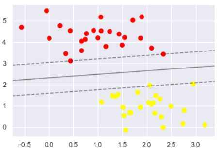
这条线就是我们希望得到的决策边界啦
观察发现有3个点做了特殊的标记,它们恰好都是边界上的点
它们就是我们的support vectors(支持向量)
在Scikit-Learn中, 它们存储在这个位置 support_vectors_(一个属性)
model.support_vectors_
array([[0.44359863, 3.11530945],
       [2.33812285, 3.43116792],
       [2.06156753, 1.96918596]])
原文:https://www.cnblogs.com/shijieli/p/11910465.html