2016-10-21
There are 32,000+ datasets at NASA, and NASA is interested in understanding the connections between these datasets and also connections to other important datasets at other government organizations outside of NASA. Metadata about the NASA datasets is available online in JSON format. Let’s look at this metadata, specifically in this report the description and keyword fields. Let’s use topic modeling to classify the description fields and connect that to the keywords.
Topic modeling is a method for unsupervised classification of documents; this method models each document as a mixture of topics and each topic as a mixture of words. The kind of method I’ll be using here for topic modeling is called latent Dirichlet allocation (LDA) but there are other possibilities for fitting a topic model. In the context here, each data set description is a document; we are going to see if we can fit model these description texts as a mixture of topics.
Let’s download the metadata for the 32,000+ NASA datasets and set up data frames for the descriptions and keywords, similarly to my last exploration.
library(jsonlite)
library(dplyr)
library(tidyr)
metadata <- fromJSON("https://data.nasa.gov/data.json")
names(metadata$dataset)
## [1] "_id" "@type" "accessLevel" "accrualPeriodicity"
## [5] "bureauCode" "contactPoint" "description" "distribution"
## [9] "identifier" "issued" "keyword" "landingPage"
## [13] "language" "modified" "programCode" "publisher"
## [17] "spatial" "temporal" "theme" "title"
## [21] "license" "isPartOf" "references" "rights"
## [25] "describedBy"nasadesc <- data_frame(id = metadata$dataset$`_id`$`$oid`, desc = metadata$dataset$description)
nasakeyword <- data_frame(id = metadata$dataset$`_id`$`$oid`,
keyword = metadata$dataset$keyword) %>%
unnest(keyword)
nasakeyword <- nasakeyword %>% mutate(keyword = toupper(keyword))Just to check on things, what are the most common keywords?
nasakeyword %>% group_by(keyword) %>% count(sort = TRUE)## # A tibble: 1,616 x 2
## keyword n
## <chr> <int>
## 1 EARTH SCIENCE 14386
## 2 OCEANS 10033
## 3 PROJECT 7463
## 4 OCEAN OPTICS 7324
## 5 ATMOSPHERE 7323
## 6 OCEAN COLOR 7270
## 7 COMPLETED 6452
## 8 ATMOSPHERIC WATER VAPOR 3142
## 9 LAND SURFACE 2720
## 10 BIOSPHERE 2449
## # ... with 1,606 more rowsTo do the topic modeling, we need to make a DocumentTermMatrix, a special kind of matrix from the tm package (of course, there is just a general concept of a “document-term matrix”). Rows correspond to documents (description texts in our case) and columns correspond to terms (i.e., words); it is a sparse matrix and the values are word counts (although they also can be tf-idf).
Let’s clean up the text a bit using stop words to remove some of the nonsense “words” leftover from HTML or other character encoding.
library(tidytext)
mystop_words <- bind_rows(stop_words,
                          data_frame(word = c("nbsp", "amp", "gt", "lt",
                                              "timesnewromanpsmt", "font",
                                              "td", "li", "br", "tr", "quot",
                                              "st", "img", "src", "strong",
                                              as.character(1:10)),
                                     lexicon = rep("custom", 25)))
word_counts <- nasadesc %>% unnest_tokens(word, desc) %>%
        anti_join(mystop_words) %>%
        count(id, word, sort = TRUE) %>%
        ungroup()
word_counts
## # A tibble: 1,909,215 x 3
## id word n
## <chr> <chr> <int>
## 1 55942a8ec63a7fe59b4986ef suit 82
## 2 55942a8ec63a7fe59b4986ef space 69
## 3 56cf5b00a759fdadc44e564a data 41
## 4 56cf5b00a759fdadc44e564a leak 40
## 5 56cf5b00a759fdadc44e564a tree 39
## 6 55942a8ec63a7fe59b4986ef pressure 34
## 7 55942a8ec63a7fe59b4986ef system 34
## 8 55942a89c63a7fe59b4982d9 em 32
## 9 55942a8ec63a7fe59b4986ef al 32
## 10 55942a8ec63a7fe59b4986ef human 31
## # ... with 1,909,205 more rowsNow let’s make the DocumentTermMatrix.
desc_dtm <- word_counts %>%
  cast_dtm(id, word, n)
desc_dtm
## <<DocumentTermMatrix (documents: 32003, terms: 35911)>>
## Non-/sparse entries: 1909215/1147350518
## Sparsity : 100%
## Maximal term length: 166
## Weighting : term frequency (tf)Now let’s use the topicmodels package to create an LDA model. How many topics will we tell the algorithm to make? This is a question much like in kk-means clustering; we don’t really know ahead of time. We can try a few different values and see how the model is doing in fitting our text. Let’s start with 8 topics.
library(topicmodels)
desc_lda <- LDA(desc_dtm, k = 8, control = list(seed = 1234))
desc_lda
## A LDA_VEM topic model with 8 topics.We have done it! We have modeled topics! This is a stochastic algorithm that could have different results depending on where the algorithm starts, so I need to put a seed for reproducibility. We’ll need to see how robust the topic modeling is eventually.
Let’s use the amazing/wonderful broom package to tidy the models, and see what we can find out.
library(broom)
tidy_lda <- tidy(desc_lda)
tidy_lda
## # A tibble: 287,288 x 3
## topic term beta
## <int> <chr> <dbl>
## 1 1 suit 2.591273e-40
## 2 2 suit 9.085227e-61
## 3 3 suit 1.620165e-61
## 4 4 suit 2.081683e-64
## 5 5 suit 9.507092e-05
## 6 6 suit 5.747629e-04
## 7 7 suit 1.808279e-63
## 8 8 suit 4.545037e-40
## 9 1 space 2.332248e-05
## 10 2 space 2.641815e-40
## # ... with 287,278 more rowsThe column ββ tells us the probability of that term being generated from that topic for that document. Notice that some of very, very low, and some are not so low.
What are the top 5 terms for each topic?
top_terms <- tidy_lda %>%
  group_by(topic) %>%
  top_n(10, beta) %>%
  ungroup() %>%
  arrange(topic, -beta)

top_terms
## # A tibble: 80 x 3
## topic term beta
## <int> <chr> <dbl>
## 1 1 data 0.047596842
## 2 1 set 0.014857522
## 3 1 soil 0.013231077
## 4 1 land 0.007874196
## 5 1 files 0.007835032
## 6 1 moisture 0.007799017
## 7 1 surface 0.006913904
## 8 1 file 0.006495391
## 9 1 collected 0.006350559
## 10 1 measurements 0.005521037
## # ... with 70 more rowsLet’s look at this visually.
library(ggplot2)
library(ggstance)
library(ggthemes)
ggplot(top_terms, aes(beta, term, fill = as.factor(topic))) +
        geom_barh(stat = "identity", show.legend = FALSE, alpha = 0.8) +
        labs(title = "Top 10 Terms in Each LDA Topic",
             subtitle = "Topic modeling of NASA metadata description field texts",
             caption = "NASA metadata from https://data.nasa.gov/data.json",
             y = NULL, x = "beta") +
        facet_wrap(~topic, ncol = 2, scales = "free") +
        theme_tufte(base_family = "Arial", base_size = 13, ticks = FALSE) +
        scale_x_continuous(expand=c(0,0)) +
        theme(strip.text=element_text(hjust=0)) +
        theme(plot.caption=element_text(size=9))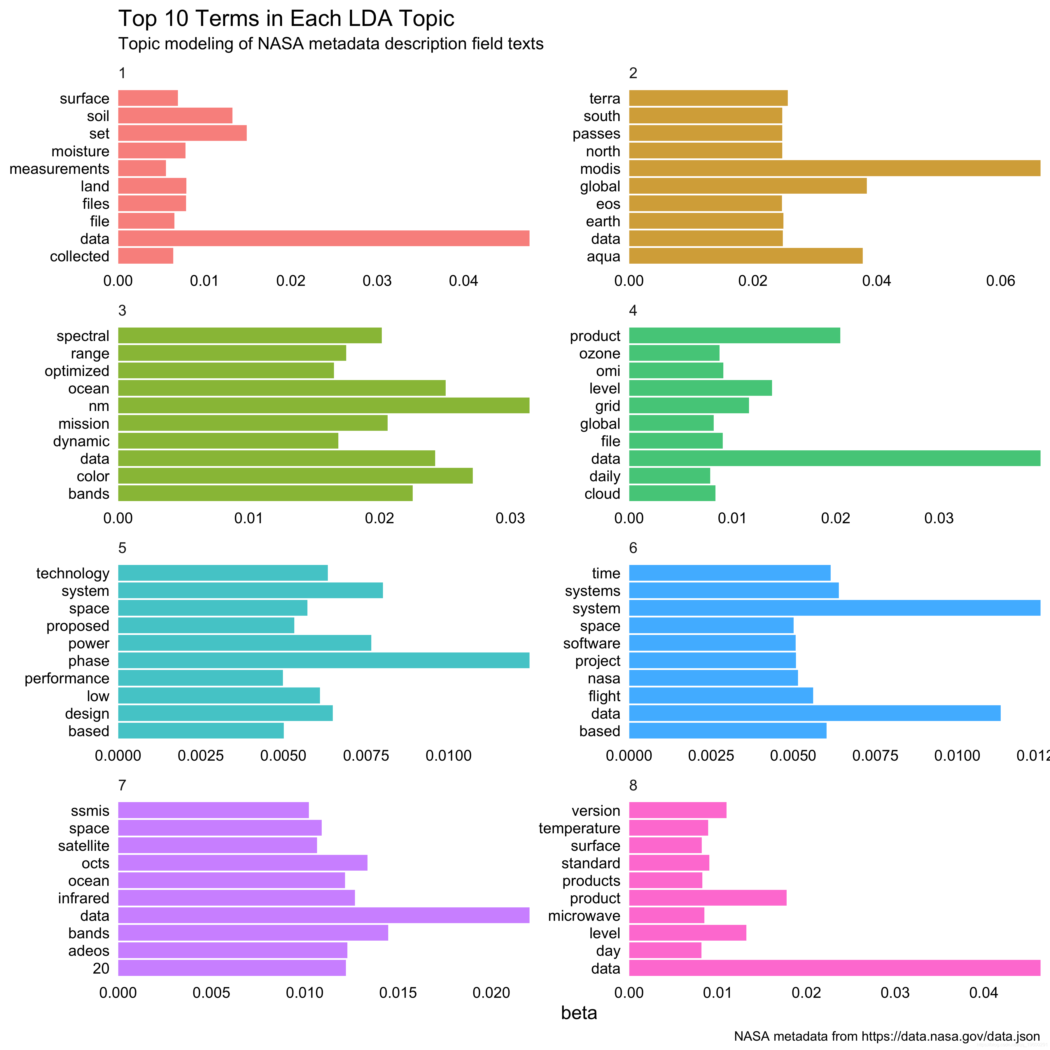
![]() ?
?
We can see what a dominant word “data” is in these description texts. There do appear to be meaningful differences between these collections of terms, though, from terms about soil and land to terms about design, systems, and technology. Further exploration is definitely needed to find the right number of topics and to do a better job here. Also, could the title and description words be combined for topic modeling?
Let’s find out which topics are associated with which description fields (i.e., documents).
lda_gamma <- tidy(desc_lda, matrix = "gamma")
lda_gamma
## # A tibble: 256,024 x 3
## document topic gamma
## <chr> <int> <dbl>
## 1 55942a8ec63a7fe59b4986ef 1 7.315366e-02
## 2 56cf5b00a759fdadc44e564a 1 9.933126e-02
## 3 55942a89c63a7fe59b4982d9 1 1.707524e-02
## 4 56cf5b00a759fdadc44e55cd 1 4.273013e-05
## 5 55942a89c63a7fe59b4982c6 1 1.257880e-04
## 6 55942a86c63a7fe59b498077 1 1.078338e-04
## 7 56cf5b00a759fdadc44e56f8 1 4.208647e-02
## 8 55942a8bc63a7fe59b4984b5 1 8.198155e-05
## 9 55942a6ec63a7fe59b496bf7 1 1.042996e-01
## 10 55942a8ec63a7fe59b4986f6 1 5.475847e-05
## # ... with 256,014 more rowsThe column γγ here is the probability that each document belongs in each topic. Notice that some are very low and some are higher. How are the probabilities distributed?
ggplot(lda_gamma, aes(gamma, fill = as.factor(topic))) +
        geom_histogram(alpha = 0.8, show.legend = FALSE) +
        facet_wrap(~topic, ncol = 4) +
        scale_y_log10() +
        labs(title = "Distribution of Probability for Each Topic",
             subtitle = "Topic modeling of NASA metadata description field texts",
             caption = "NASA metadata from https://data.nasa.gov/data.json",
             y = NULL, x = "gamma") +
        theme_minimal(base_family = "Arial", base_size = 13) +
        theme(strip.text=element_text(hjust=0)) +
        theme(plot.caption=element_text(size=9))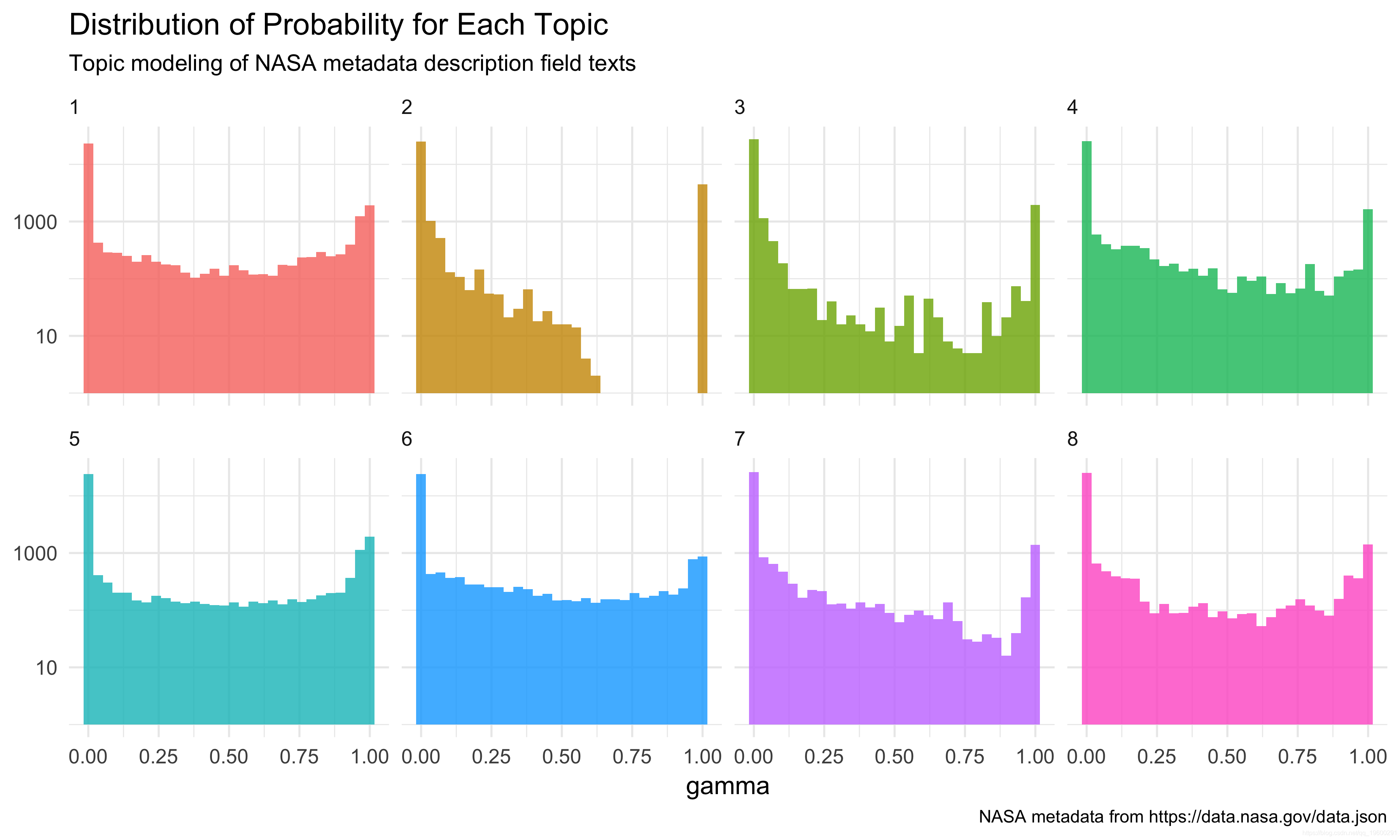
![]() ?
?
The y-axis is plotted here on a log scale so we can see something. Most documents are getting sorted into one of these topics with decent probability; lots of documents are getting sorted into topics 2, and documents are being sorted into topics 1 and 5 (6?) less cleanly. Some topics have fewer documents. For any individual document, we could find the topic that it has the highest probability of belonging to.
Let’s connect these topic models with the keywords and see what happens. Let’s join this dataframe to the keywords and see which keywords are associated with which topic.
lda_gamma <- full_join(lda_gamma, nasakeyword, by = c("document" = "id"))
lda_gamma
## # A tibble: 1,012,727 x 4
## document topic gamma keyword
## <chr> <int> <dbl> <chr>
## 1 55942a8ec63a7fe59b4986ef 1 7.315366e-02 JOHNSON SPACE CENTER
## 2 55942a8ec63a7fe59b4986ef 1 7.315366e-02 PROJECT
## 3 55942a8ec63a7fe59b4986ef 1 7.315366e-02 COMPLETED
## 4 56cf5b00a759fdadc44e564a 1 9.933126e-02 DASHLINK
## 5 56cf5b00a759fdadc44e564a 1 9.933126e-02 AMES
## 6 56cf5b00a759fdadc44e564a 1 9.933126e-02 NASA
## 7 55942a89c63a7fe59b4982d9 1 1.707524e-02 GODDARD SPACE FLIGHT CENTER
## 8 55942a89c63a7fe59b4982d9 1 1.707524e-02 PROJECT
## 9 55942a89c63a7fe59b4982d9 1 1.707524e-02 COMPLETED
## 10 56cf5b00a759fdadc44e55cd 1 4.273013e-05 DASHLINK
## # ... with 1,012,717 more rowsLet’s keep each document that was modeled as belonging to a topic with a probability >0.9>0.9, and then find the top keywords for each topic.
top_keywords <- lda_gamma %>% filter(gamma > 0.9) %>%
        group_by(topic, keyword) %>%
        count(keyword, sort = TRUE)
top_keywords
## Source: local data frame [1,240 x 3]
## Groups: topic [8]
##
## topic keyword n
## <int> <chr> <int>
## 1 2 OCEAN COLOR 4480
## 2 2 OCEAN OPTICS 4480
## 3 2 OCEANS 4480
## 4 1 EARTH SCIENCE 3469
## 5 5 PROJECT 3464
## 6 5 COMPLETED 3057
## 7 8 EARTH SCIENCE 2229
## 8 3 OCEAN COLOR 1968
## 9 3 OCEAN OPTICS 1968
## 10 3 OCEANS 1968
## # ... with 1,230 more rowsLet’s do a visualization for these as well.
top_keywords <- top_keywords %>%
        top_n(10, n)
ggplot(top_keywords, aes(n, keyword, fill = as.factor(topic))) +
        geom_barh(stat = "identity", show.legend = FALSE, alpha = 0.8) +
        labs(title = "Top 10 Keywords for Each LDA Topic",
             subtitle = "Topic modeling of NASA metadata description field texts",
             caption = "NASA metadata from https://data.nasa.gov/data.json",
             y = NULL, x = "Number of documents") +
        facet_wrap(~topic, ncol = 2, scales = "free") +
        theme_tufte(base_family = "Arial", base_size = 13, ticks = FALSE) +
        scale_x_continuous(expand=c(0,0)) +
        theme(strip.text=element_text(hjust=0)) +
        theme(plot.caption=element_text(size=9))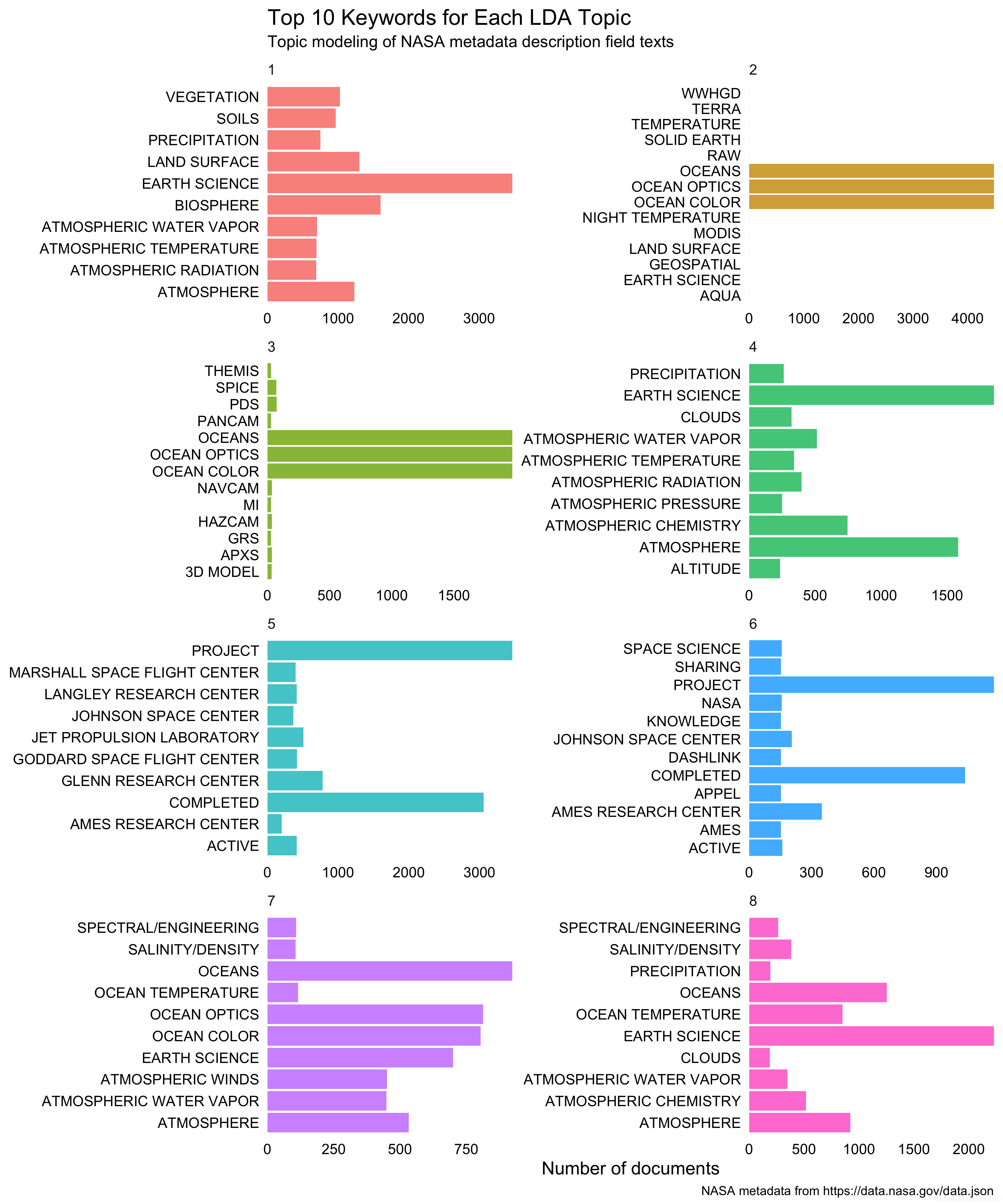
![]() ?
?
These are really interesting combinations of keywords. I am not confident in this particular number of topics, or how robust this modeling might be (not tested yet), but this looks very interesting and is a first step!
NASA Metadata: Topic Modeling of Description Texts
原文:https://www.cnblogs.com/tecdat/p/12035890.html