茅台股票分析
代码实现:
1.使用tushare包获取某股票的历史行情数据
import tushare as ts
import pandas as pd
from pandas import Series,DataFrame

# 使用tushare包获取某股票的历史行情数据
df = ts.get_k_data('600519',start='1988-01-01')
# 将获取的数据写入到本地进行持久化存储
df.to_csv('./maotai.csv')

# 将本地文本文件中的数据读取加载到DataFrame中
df = pd.read_csv('./maotai.csv')
df.head(10)

# 将Unnamed: 0为无用的列删除
df.drop(labels='Unnamed: 0',axis=1,inplace=True)
df.head(5)  # 显示前五条,不写5默认也是显示的前5条,inplace是判断是否用新表替换原表

# 将date列转成时间序列类型
df['date'] = pd.to_datetime(df['date'])

# 将date列作为元数据的行索引
df.set_index(df['date'],inplace=True)

# 删除原date列
df.drop(labels='date',axis=1,inplace=True)
df.head()
2.输出该股票所有收盘比开盘上涨3%以上的日期。
# 伪代码:(收盘-开盘)/开盘  > 0.03
(df['close'] - df['open'])/df['open'] > 0.03

# boolean可以作为df的行索引
df.loc[[True,False,True]]
df.loc[(df['close'] - df['open'])/df['open'] > 0.03]

df.loc[(df['close'] - df['open'])/df['open'] > 0.03].index
3.输出该股票所有开盘比前日收盘跌幅超过2%的日期
#伪代码:(开盘-前日收盘)/前日收盘  < -0.02

# 将收盘/close列下移一位,这样可以将open和close作用到一行,方便比较
(df['open'] - df['close'].shift(1))/df['close'].shift(1) < -0.02

# boolean作为df的行索引
df.loc[(df['open'] - df['close'].shift(1))/df['close'].shift(1) < -0.02]

df.loc[(df['open'] - df['close'].shift(1))/df['close'].shift(1) < -0.02].index

# shift(1):可以让一个Series中的数据整体下移一位
4.假如从2010年1月1日开始,每月第一个交易日买入1手股票,每年最后一个交易日卖出所有股票,到今天为止,收益如何?
分析:
买入:一个完整的年需要买12次股票,一次买入一手(100支),一个完整的年需要买入1200支股票
卖出:一个完整的年卖一次,一次卖出1200只股票
代码实现:
# 将2010-1-1 - 今天对应的交易数据取出
data = df['2010':'2019']
data.head()

# 数据的重新取样,将每个月第一个交易日的数据拿到
data_monthly = data.resample('M').first()

# 一共花了多少钱
cost_money = (data_monthly['open']*100).sum()

# 卖出股票入手多少钱,将每年的最后一个交易日的数据拿到
data_yeasly = data.resample('A').last()[:-1]
recv_money = (data_yeasly['open']*1200).sum()

# 19年手里剩余股票的价值也要计算到收益中
last_money = 1200*data['close'][-1]

# 最后总收益如下:
last_monry + recv_money - cost_monry双均线策略分析
代码实现
1.使用tushare包获取某股票的历史行情数据
import tushare as ts
import pandas as pd

# 调用tushare接口,分析股票历史数据
df = ts.get_k_data('601318',start='1990-01-01')


# 数据的预处理
# 将date列转换成时间序列
df['date'] = pd.to_datetime(df['date'])
# 将新的date时间序列,设置成索引,并替换原数据
df.set_index(df['date'],inplace=True)
# 删除掉原来的date列
df.drop(labels='date',axis=1,inplace=True)
# 取2010-2019区间的数据,2010之前的数据有NaN数据,会造成统计结果不准确
df = df['2010':'2019']
2.计算该股票历史数据的5日均线和30日均线
# rolling是第几个5天的值,mean()取均值
df['ma5'] = df['close'].rolling(5).mean()
df['ma30'] = df['close'].rolling(30).mean()
3.可视化历史数据两条均线
# 可视化历史数据两条均线,c代表颜色
import matplotlib.pyplot as plt
df_p = df[:300]
plt.plot(df_p.index,df_p['ma5'],c='red')
plt.plot(df_p.index,df_p['ma30'],c='blue')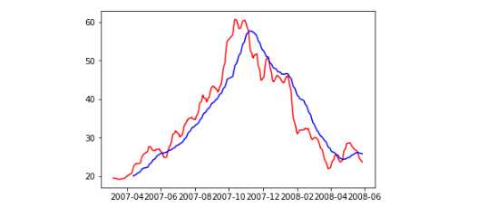
4.分析输出所有金叉日期和死叉日期
# True:短期均线 低于 长期均线
# False:短期均线 高于 长期均线
# True ---> False 的过渡,对应的点是金叉
# False ---> True 的过渡,对应的点是死叉
sr1 = df['ma5'] < df['ma30']
sr2 = df['ma5'] >= df['ma30']

# 捕获死叉所有的日期   按位与:&
death_date = df.loc[sr1 & sr2.shift(1)].index

# 捕获所有的金叉日期  按位或:|   取反:~
golden_date = df.loc[~(sr1 | sr2.shift(1))].index
5.如果假如从开始,初始资金为100000元,金叉尽量买入,死叉全部卖出,则到今天为止,炒股收益率如何?
first_money = 100000 # 不变
money = first_money  #可变的
hold = 0  # 目前所持有股票的数量(单位:支)

from pandas import Series
s1 = Series(1,index=golden_date)  # 存储的是为金叉日期,用1表示
s2 = Series(0,index=death_date)   # 死叉日期,0表示
s = s1.append(s2)
s = s.sort_index()

# 使用开盘价进行股票的买卖
for i in range(0,len(s)): # 2010-07-07
    # 买入或卖出股票的单价:p
    p = df['open'][s.index[i]]
    if s[i] == 1: # 金叉日期:买入股票
        buy = money // (p*100)  # 买了多少手
        hold = buy * 100
        money -= buy*100*p
    else:  # 卖出
        money += hold * p
        hold = 0

money += hold * df['open'][-1]
result = money - first_money
print(result)
数据分析04 /基于pandas的DateFrame进行股票分析、双均线策略制定
原文:https://www.cnblogs.com/liubing8/p/12037238.html