假设现在有一些数据点,我们用
一条直线对这些点进行拟合(该线称为最佳拟合直线),这个拟合过程就称作回归。利用Logistic
回归进行分类的主要思想是:根据现有数据对分类边界线建立回归公式,以此进行分类。这里的
“ 回归” 一词源于最佳拟合,表示要找到最佳拟合参数集。
训练分类器时的做法就是寻找最佳拟合参数,使用的是最优化算法。

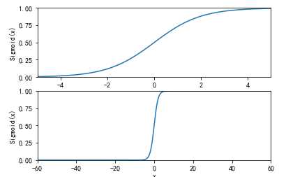
基于Logistic回归和Sigmoid函数的分类


import sys
from pylab import *

t = arange(-60.0, 60.3, 0.1)
s = 1/(1 + exp(-t))
ax = subplot(211)
ax.plot(t,s)
ax.axis([-5,5,0,1])
plt.xlabel(‘x‘)
plt.ylabel(‘Sigmoid(x)‘)
ax = subplot(212)
ax.plot(t,s)
ax.axis([-60,60,0,1])
plt.xlabel(‘x‘)
plt.ylabel(‘Sigmoid(x)‘)
show()
基于最优化方法的最佳回归系数确定

梯度上升法
梯度上升法基于的思想是:要找到某函数的
最大值,最好的方法是沿着该函数的梯度方向探寻。
import matplotlib
import numpy as np
import matplotlib.cm as cm
import matplotlib.mlab as mlab
import matplotlib.pyplot as plt

leafNode = dict(boxstyle="round4", fc="0.8")
arrow_args = dict(arrowstyle="<-")

matplotlib.rcParams[‘xtick.direction‘] = ‘out‘
matplotlib.rcParams[‘ytick.direction‘] = ‘out‘

delta = 0.025
x = np.arange(-2.0, 2.0, delta)
y = np.arange(-2.0, 2.0, delta)
X, Y = np.meshgrid(x, y)
Z1 = -((X-1)**2)
Z2 = -(Y**2)
#Z1 = mlab.bivariate_normal(X, Y, 1.0, 1.0, 0.0, 0.0)
#Z2 = mlab.bivariate_normal(X, Y, 1.5, 0.5, 1, 1)
# difference of Gaussians
Z = 1.0 * (Z2 + Z1)+5.0

# Create a simple contour plot with labels using default colors.  The
# inline argument to clabel will control whether the labels are draw
# over the line segments of the contour, removing the lines beneath
# the label
plt.figure()
CS = plt.contour(X, Y, Z)
plt.annotate(‘‘, xy=(0.05, 0.05),  xycoords=‘axes fraction‘,xytext=(0.2,0.2), textcoords=‘axes fraction‘,va="center", ha="center", bbox=leafNode, arrowprops=arrow_args )
plt.text(-1.9, -1.8, ‘P0‘)

plt.annotate(‘‘, xy=(0.2,0.2),  xycoords=‘axes fraction‘,xytext=(0.35,0.3), textcoords=‘axes fraction‘,va="center", ha="center", bbox=leafNode, arrowprops=arrow_args )
plt.text(-1.35, -1.23, ‘P1‘)

plt.annotate(‘‘, xy=(0.35,0.3),  xycoords=‘axes fraction‘,xytext=(0.45,0.35), textcoords=‘axes fraction‘,va="center", ha="center", bbox=leafNode, arrowprops=arrow_args )
plt.text(-0.7, -0.8, ‘P2‘)
plt.text(-0.3, -0.6, ‘P3‘)

plt.clabel(CS, inline=1, fontsize=10)
plt.title(‘Gradient Ascent‘)
plt.xlabel(‘x‘)
plt.ylabel(‘y‘)
plt.show()
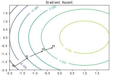

可以看到,梯度算子总是指向函数值增长
最快的方向。这里所说的是移动方向,而未提到移动量的大小。该量值称为步长,记做a用向
量来表示的话,梯度算法的迭代公式如下:


训练算法:使用梯度上升找到最佳参数
from numpy import *

def loadDataSet():
    dataMat = []; labelMat = []
    fr = open(‘testSet.txt‘)
    for line in fr.readlines():
        lineArr = line.strip().split()
        dataMat.append([1.0, float(lineArr[0]), float(lineArr[1])])
        labelMat.append(int(lineArr[2]))
    return dataMat,labelMat

def sigmoid(inX):
    return 1.0/(1+exp(-inX))

def gradAscent(dataMatIn, classLabels):
    dataMatrix = mat(dataMatIn)             #convert to NumPy matrix
    labelMat = mat(classLabels).transpose() #convert to NumPy matrix
    m,n = shape(dataMatrix)
    alpha = 0.001
    maxCycles = 500
    weights = ones((n,1))
    for k in range(maxCycles):              #heavy on matrix operations
        h = sigmoid(dataMatrix*weights)     #matrix mult
        error = (labelMat - h)              #vector subtraction
        weights = weights + alpha * dataMatrix.transpose()* error #matrix mult
    return weights
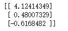
dataMat,labelMat = loadDataSet()
weights = gradAscent(dataMat,labelMat)
print(weights)
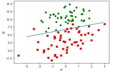
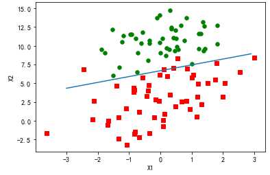
分析数据:画出决策边界
上面已经解出了一组回归系数,它确定了不同类别数据之间的分隔线。
import matplotlib
import matplotlib.pyplot as plt

from numpy import *
from matplotlib.patches import Rectangle

def loadDataSet():
    dataMat = []
    labelMat = []
    fr = open(‘F:\\machinelearninginaction\\Ch05\\testSet.txt‘)
    for line in fr.readlines():
        lineArr = line.strip().split()
        dataMat.append([1.0, float(lineArr[0]), float(lineArr[1])])
        labelMat.append(int(lineArr[2]))
    return dataMat,labelMat

def sigmoid(inX):
    return 1.0/(1+exp(-inX))

def stocGradAscent0(dataMatrix, classLabels):
    m,n = shape(dataMatrix)
    alpha = 0.01
    weights = ones(n)   #initialize to all ones
    for i in range(m):
        h = sigmoid(sum(dataMatrix[i]*weights))
        error = classLabels[i] - h
        weights = weights + alpha * error * dataMatrix[i]
    return weights

def gradAscent(dataMatIn, classLabels):
    dataMatrix = mat(dataMatIn)             #convert to NumPy matrix
    labelMat = mat(classLabels).transpose() #convert to NumPy matrix
    m,n = shape(dataMatrix)
    alpha = 0.001
    maxCycles = 500
    weights = ones((n,1))
    for k in range(maxCycles):              #heavy on matrix operations
        h = sigmoid(dataMatrix*weights)     #matrix mult
        error = (labelMat - h)              #vector subtraction
        weights = weights + alpha * dataMatrix.transpose()* error #matrix mult
    return weights

dataMat,labelMat=loadDataSet()
dataArr = array(dataMat)
weights = gradAscent(dataArr,labelMat)

n = shape(dataArr)[0] #number of points to create
xcord1 = []
ycord1 = []
xcord2 = []
ycord2 = []

markers =[]
colors =[]
for i in range(n):
    if int(labelMat[i])== 1:
        xcord1.append(dataArr[i,1]); ycord1.append(dataArr[i,2])
    else:
        xcord2.append(dataArr[i,1]); ycord2.append(dataArr[i,2])

fig = plt.figure()
ax = fig.add_subplot(111)
#ax.scatter(xcord,ycord, c=colors, s=markers)
type1 = ax.scatter(xcord1, ycord1, s=30, c=‘red‘, marker=‘s‘)
type2 = ax.scatter(xcord2, ycord2, s=30, c=‘green‘)
x = arange(-3.0, 3.0, 0.1)
#weights = [-2.9, 0.72, 1.29]
#weights = [-5, 1.09, 1.42]
weights = [13.03822793,   1.32877317,  -1.96702074]
weights = [4.12,   0.48,  -0.6168]
y = (-weights[0]-weights[1]*x)/weights[2]
type3 = ax.plot(x, y)
#ax.legend([type1, type2, type3], ["Did Not Like", "Liked in Small Doses", "Liked in Large Doses"], loc=2)
#ax.axis([-5000,100000,-2,25])
plt.xlabel(‘X1‘)
plt.ylabel(‘X2‘)
plt.show()
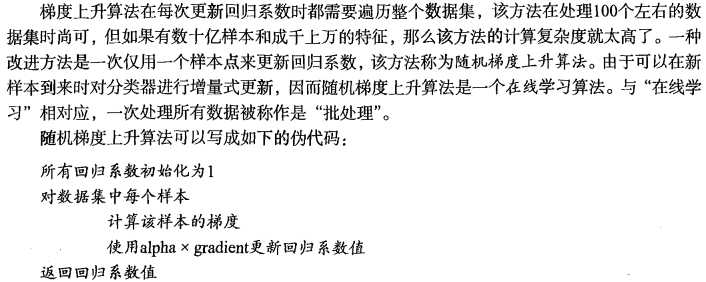
训练算法:随机梯度上升
def stocGradAscent0(dataMatrix, classLabels):
    m,n = shape(dataMatrix)
    alpha = 0.01
    weights = ones(n)   #initialize to all ones
    for i in range(m):
        h = sigmoid(sum(dataMatrix[i]*weights))
        error = classLabels[i] - h
        weights = weights + alpha * error * dataMatrix[i]
    return weights
import matplotlib
import matplotlib.pyplot as plt

from numpy import *
from matplotlib.patches import Rectangle

def loadDataSet():
    dataMat = []
    labelMat = []
    fr = open(‘F:\\machinelearninginaction\\Ch05\\testSet.txt‘)
    for line in fr.readlines():
        lineArr = line.strip().split()
        dataMat.append([1.0, float(lineArr[0]), float(lineArr[1])])
        labelMat.append(int(lineArr[2]))
    return dataMat,labelMat

def sigmoid(inX):
    return 1.0/(1+exp(-inX))

def stocGradAscent0(dataMatrix, classLabels):
    m,n = shape(dataMatrix)
    alpha = 0.01
    weights = ones(n)   #initialize to all ones
    for i in range(m):
        h = sigmoid(sum(dataMatrix[i]*weights))
        error = classLabels[i] - h
        weights = weights + alpha * error * dataMatrix[i]
    return weights

def gradAscent(dataMatIn, classLabels):
    dataMatrix = mat(dataMatIn)             #convert to NumPy matrix
    labelMat = mat(classLabels).transpose() #convert to NumPy matrix
    m,n = shape(dataMatrix)
    alpha = 0.001
    maxCycles = 500
    weights = ones((n,1))
    for k in range(maxCycles):              #heavy on matrix operations
        h = sigmoid(dataMatrix*weights)     #matrix mult
        error = (labelMat - h)              #vector subtraction
        weights = weights + alpha * dataMatrix.transpose()* error #matrix mult
    return weights

dataMat,labelMat=loadDataSet()
dataArr = array(dataMat)
weights = stocGradAscent0(dataArr,labelMat)

n = shape(dataArr)[0] #number of points to create
xcord1 = []
ycord1 = []
xcord2 = []
ycord2 = []

markers =[]
colors =[]
for i in range(n):
    if int(labelMat[i])== 1:
        xcord1.append(dataArr[i,1]); ycord1.append(dataArr[i,2])
    else:
        xcord2.append(dataArr[i,1]); ycord2.append(dataArr[i,2])

fig = plt.figure()
ax = fig.add_subplot(111)
#ax.scatter(xcord,ycord, c=colors, s=markers)
type1 = ax.scatter(xcord1, ycord1, s=30, c=‘red‘, marker=‘s‘)
type2 = ax.scatter(xcord2, ycord2, s=30, c=‘green‘)
x = arange(-3.0, 3.0, 0.1)
#weights = [-2.9, 0.72, 1.29]
#weights = [-5, 1.09, 1.42]
weights = [13.03822793,   1.32877317,  -1.96702074]
weights = [4.12,   0.48,  -0.6168]
y = (-weights[0]-weights[1]*x)/weights[2]
type3 = ax.plot(x, y)
#ax.legend([type1, type2, type3], ["Did Not Like", "Liked in Small Doses", "Liked in Large Doses"], loc=2)
#ax.axis([-5000,100000,-2,25])
plt.xlabel(‘X1‘)
plt.ylabel(‘X2‘)
plt.show()
import matplotlib
import matplotlib.pyplot as plt

from numpy import *
from matplotlib.patches import Rectangle

def loadDataSet():
    dataMat = []
    labelMat = []
    fr = open(‘F:\\machinelearninginaction\\Ch05\\testSet.txt‘)
    for line in fr.readlines():
        lineArr = line.strip().split()
        dataMat.append([1.0, float(lineArr[0]), float(lineArr[1])])
        labelMat.append(int(lineArr[2]))
    return dataMat,labelMat

def sigmoid(inX):
    return 1.0/(1+exp(-inX))

def stocGradAscent0(dataMatrix, classLabels):
    m,n = shape(dataMatrix)
    alpha = 0.5
    weights = ones(n)   #initialize to all ones
    weightsHistory=zeros((500*m,n))
    for j in range(500):
        for i in range(m):
            h = sigmoid(sum(dataMatrix[i]*weights))
            error = classLabels[i] - h
            weights = weights + alpha * error * dataMatrix[i]
            weightsHistory[j*m + i,:] = weights
    return weightsHistory

def stocGradAscent1(dataMatrix, classLabels):
    m,n = shape(dataMatrix)
    alpha = 0.4
    weights = ones(n)   #initialize to all ones
    weightsHistory=zeros((40*m,n))
    for j in range(40):
        dataIndex = range(m)
        for i in range(m):
            alpha = 4/(1.0+j+i)+0.01
            randIndex = int(random.uniform(0,len(dataIndex)))
            h = sigmoid(sum(dataMatrix[randIndex]*weights))
            error = classLabels[randIndex] - h
            #print error
            weights = weights + alpha * error * dataMatrix[randIndex]
            weightsHistory[j*m + i,:] = weights
#             del(dataIndex[randIndex])
    print(weights)
    return weightsHistory


dataMat,labelMat=loadDataSet()
dataArr = array(dataMat)
myHist = stocGradAscent1(dataArr,labelMat)


n = shape(dataArr)[0] #number of points to create
xcord1 = []
ycord1 = []
xcord2 = []
ycord2 = []

markers =[]
colors =[]


fig = plt.figure()
ax = fig.add_subplot(311)
type1 = ax.plot(myHist[:,0])
plt.ylabel(‘X0‘)
ax = fig.add_subplot(312)
type1 = ax.plot(myHist[:,1])
plt.ylabel(‘X1‘)
ax = fig.add_subplot(313)
type1 = ax.plot(myHist[:,2])
plt.xlabel(‘iteration‘)
plt.ylabel(‘X2‘)
plt.show()
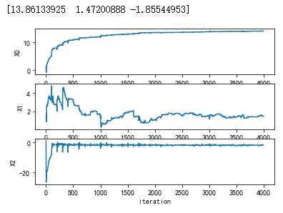

值 得注意的是,在大的波动停止后,还有一些小的周期性波动。不难理解,产生这种现象的原因是
存在一些不能正确分类的样本点(数据集并非线性可分),在每次迭代时会引发系数的剧烈改变。
我们期望算法能避免来回波动,从而收敛到某个值。另外,收敛速度也需要加快。
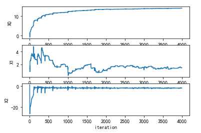
改进的随机梯度上升算法
def stocGradAscent1(dataMatrix, classLabels, numIter=150):
    m,n = shape(dataMatrix)
    weights = ones(n)   #initialize to all ones
    for j in range(numIter):
        dataIndex = range(m)
        for i in range(m):
            alpha = 4/(1.0+j+i)+0.0001    #apha decreases with iteration, does not
            randIndex = int(random.uniform(0,len(dataIndex)))#go to 0 because of the constant
            h = sigmoid(sum(dataMatrix[randIndex]*weights))
            error = classLabels[randIndex] - h
            weights = weights + alpha * error * dataMatrix[randIndex]
            del(dataIndex[randIndex])
    return weights
import matplotlib
import matplotlib.pyplot as plt

from numpy import *
from matplotlib.patches import Rectangle

def loadDataSet():
    dataMat = []
    labelMat = []
    fr = open(‘F:\\machinelearninginaction\\Ch05\\testSet.txt‘)
    for line in fr.readlines():
        lineArr = line.strip().split()
        dataMat.append([1.0, float(lineArr[0]), float(lineArr[1])])
        labelMat.append(int(lineArr[2]))
    return dataMat,labelMat

def sigmoid(inX):
    return 1.0/(1+exp(-inX))

def stocGradAscent0(dataMatrix, classLabels):
    m,n = shape(dataMatrix)
    alpha = 0.5
    weights = ones(n)   #initialize to all ones
    weightsHistory=zeros((500*m,n))
    for j in range(500):
        for i in range(m):
            h = sigmoid(sum(dataMatrix[i]*weights))
            error = classLabels[i] - h
            weights = weights + alpha * error * dataMatrix[i]
            weightsHistory[j*m + i,:] = weights
    return weightsHistory

def stocGradAscent1(dataMatrix, classLabels):
    m,n = shape(dataMatrix)
    alpha = 0.4
    weights = ones(n)   #initialize to all ones
    weightsHistory=zeros((40*m,n))
    for j in range(40):
        dataIndex = range(m)
        for i in range(m):
            alpha = 4/(1.0+j+i)+0.01
            randIndex = int(random.uniform(0,len(dataIndex)))
            h = sigmoid(sum(dataMatrix[randIndex]*weights))
            error = classLabels[randIndex] - h
            #print error
            weights = weights + alpha * error * dataMatrix[randIndex]
            weightsHistory[j*m + i,:] = weights
#             del(dataIndex[randIndex])
    print(weights)
    return weightsHistory


dataMat,labelMat=loadDataSet()
dataArr = array(dataMat)
myHist = stocGradAscent1(dataArr,labelMat)


n = shape(dataArr)[0] #number of points to create
xcord1 = []
ycord1 = []
xcord2 = []
ycord2 = []

markers =[]
colors =[]


fig = plt.figure()
ax = fig.add_subplot(311)
type1 = ax.plot(myHist[:,0])
plt.ylabel(‘X0‘)
ax = fig.add_subplot(312)
type1 = ax.plot(myHist[:,1])
plt.ylabel(‘X1‘)
ax = fig.add_subplot(313)
type1 = ax.plot(myHist[:,2])
plt.xlabel(‘iteration‘)
plt.ylabel(‘X2‘)
plt.show()
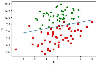
import matplotlib
import matplotlib.pyplot as plt

from numpy import *
from matplotlib.patches import Rectangle

def loadDataSet():
    dataMat = []
    labelMat = []
    fr = open(‘F:\\machinelearninginaction\\Ch05\\testSet.txt‘)
    for line in fr.readlines():
        lineArr = line.strip().split()
        dataMat.append([1.0, float(lineArr[0]), float(lineArr[1])])
        labelMat.append(int(lineArr[2]))
    return dataMat,labelMat

def sigmoid(inX):
    return 1.0/(1+exp(-inX))

def stocGradAscent0(dataMatrix, classLabels):
    m,n = shape(dataMatrix)
    alpha = 0.01
    weights = ones(n)   #initialize to all ones
    for i in range(m):
        h = sigmoid(sum(dataMatrix[i]*weights))
        error = classLabels[i] - h
        weights = weights + alpha * error * dataMatrix[i]
    return weights

def gradAscent(dataMatIn, classLabels):
    dataMatrix = mat(dataMatIn)             #convert to NumPy matrix
    labelMat = mat(classLabels).transpose() #convert to NumPy matrix
    m,n = shape(dataMatrix)
    alpha = 0.001
    maxCycles = 500
    weights = ones((n,1))
    for k in range(maxCycles):              #heavy on matrix operations
        h = sigmoid(dataMatrix*weights)     #matrix mult
        error = (labelMat - h)              #vector subtraction
        weights = weights + alpha * dataMatrix.transpose()* error #matrix mult
    return weights

def stocGradAscent1(dataMatrix, classLabels, numIter=150):
    m,n = shape(dataMatrix)
    weights = ones(n)   #initialize to all ones
    for j in range(numIter):
        dataIndex = range(m)
        for i in range(m):
            alpha = 4/(1.0+j+i)+0.0001    #apha decreases with iteration, does not
            randIndex = int(random.uniform(0,len(dataIndex)))#go to 0 because of the constant
            h = sigmoid(sum(dataMatrix[randIndex]*weights))
            error = classLabels[randIndex] - h
            weights = weights + alpha * error * dataMatrix[randIndex]
#             del(dataIndex[randIndex])
    return weights

dataMat,labelMat=loadDataSet()
dataArr = array(dataMat)
weights = stocGradAscent1(dataArr,labelMat)

n = shape(dataArr)[0] #number of points to create
xcord1 = []
ycord1 = []
xcord2 = []
ycord2 = []

markers =[]
colors =[]
for i in range(n):
    if int(labelMat[i])== 1:
        xcord1.append(dataArr[i,1]); ycord1.append(dataArr[i,2])
    else:
        xcord2.append(dataArr[i,1]); ycord2.append(dataArr[i,2])

fig = plt.figure()
ax = fig.add_subplot(111)
#ax.scatter(xcord,ycord, c=colors, s=markers)
type1 = ax.scatter(xcord1, ycord1, s=30, c=‘red‘, marker=‘s‘)
type2 = ax.scatter(xcord2, ycord2, s=30, c=‘green‘)
x = arange(-3.0, 3.0, 0.1)
#weights = [-2.9, 0.72, 1.29]
#weights = [-5, 1.09, 1.42]
weights = [13.03822793,   1.32877317,  -1.96702074]
weights = [4.12,   0.48,  -0.6168]
y = (-weights[0]-weights[1]*x)/weights[2]
type3 = ax.plot(x, y)
#ax.legend([type1, type2, type3], ["Did Not Like", "Liked in Small Doses", "Liked in Large Doses"], loc=2)
#ax.axis([-5000,100000,-2,25])
plt.xlabel(‘X1‘)
plt.ylabel(‘X2‘)
plt.show()
吴裕雄--天生自然python机器学习:Logistic回归
原文:https://www.cnblogs.com/tszr/p/12045360.html