目录
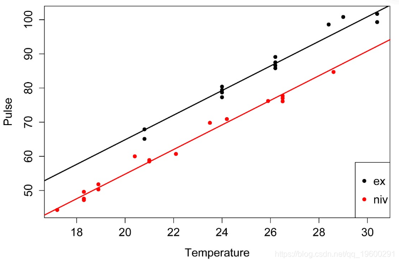
具有两个类别和II型平方和的协方差示例的分析
本示例使用II型平方和 。参数估计值在R中的计算方式不同,
Data = read.table(textConnection(Input),header=TRUE)
plot(x   = Data$Temp,
     y   = Data$Pulse,
     col = Data$Species,
     pch = 16,
     xlab = "Temperature",
     ylab = "Pulse")

legend(‘bottomright‘,
       legend = levels(Data$Species),
       col = 1:2,
       cex = 1,
       pch = 16)
Anova Table (Type II tests)


             Sum Sq Df  F value    Pr(>F)

Temp         4376.1  1 1388.839 < 2.2e-16 ***

Species       598.0  1  189.789 9.907e-14 ***

Temp:Species    4.3  1    1.357    0.2542


### Interaction is not significant, so the slope across groups

### is not different.


model.2 = lm (Pulse ~ Temp + Species,
              data = Data)

library(car)

Anova(model.2, type="II")


Anova Table (Type II tests)


          Sum Sq Df F value    Pr(>F)

Temp      4376.1  1  1371.4 < 2.2e-16 ***

Species    598.0  1   187.4 6.272e-14 ***


### The category variable (Species) is significant,

### so the intercepts among groups are different


Coefficients:

             Estimate Std. Error t value Pr(>|t|)

(Intercept)  -7.21091    2.55094  -2.827  0.00858 **

Temp          3.60275    0.09729  37.032  < 2e-16 ***

Speciesniv  -10.06529    0.73526 -13.689 6.27e-14 ***


###   but the calculated results will be identical.

### The slope estimate is the same.

### The intercept for species 1 (ex) is (intercept).

### The intercept for species 2 (niv) is (intercept) + Speciesniv.

### This is determined from the contrast coding of the Species

### variable shown below, and the fact that Speciesniv is shown in

### coefficient table above.


    niv

ex    0

niv   1
plot(x   = Data$Temp,
     y   = Data$Pulse,
     col = Data$Species,
     pch = 16,
     xlab = "Temperature",
     ylab = "Pulse")
![]() ?
?
Multiple R-squared:  0.9896,  Adjusted R-squared:  0.9888

F-statistic:  1331 on 2 and 28 DF,  p-value: < 2.2e-16
![]() ?
?
线性模型中残差的直方图。这些残差的分布应近似正态。
![]() ?
?
残差与预测值的关系图。残差应无偏且均等。
### additional model checking plots with: plot(model.2)
### alternative: library(FSA); residPlot(model.2)
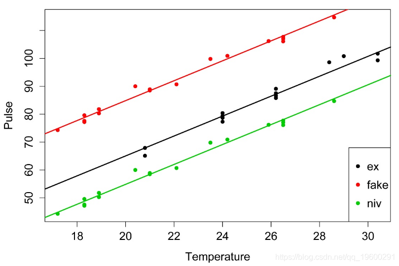
本示例使用II型平方和,并考虑具有三个组的情况。
### --------------------------------------------------------------
### Analysis of covariance, hypothetical data
### --------------------------------------------------------------


Data = read.table(textConnection(Input),header=TRUE)
plot(x   = Data$Temp,
     y   = Data$Pulse,
     col = Data$Species,
     pch = 16,
     xlab = "Temperature",
     ylab = "Pulse")

legend(‘bottomright‘,
       legend = levels(Data$Species),
       col = 1:3,
       cex = 1,
       pch = 16)
options(contrasts = c("contr.treatment", "contr.poly"))

   ### These are the default contrasts in R


Anova(model.1, type="II")


             Sum Sq Df   F value Pr(>F)

Temp         7026.0  1 2452.4187 <2e-16 ***

Species      7835.7  2 1367.5377 <2e-16 ***

Temp:Species    5.2  2    0.9126 0.4093


### Interaction is not significant, so the slope among groups

### is not different.


Anova(model.2, type="II")


          Sum Sq Df F value    Pr(>F)

Temp      7026.0  1  2462.2 < 2.2e-16 ***

Species   7835.7  2  1373.0 < 2.2e-16 ***

Residuals  125.6 44


### The category variable (Species) is significant,

### so the intercepts among groups are different


summary(model.2)


Coefficients:

             Estimate Std. Error t value Pr(>|t|)

(Intercept)  -6.35729    1.90713  -3.333  0.00175 **

Temp          3.56961    0.07194  49.621  < 2e-16 ***

Speciesfake  19.81429    0.66333  29.871  < 2e-16 ***

Speciesniv  -10.18571    0.66333 -15.355  < 2e-16 ***


### The slope estimate is the Temp coefficient.

### The intercept for species 1 (ex) is (intercept).

### The intercept for species 2 (fake) is (intercept) + Speciesfake.

### The intercept for species 3 (niv) is (intercept) + Speciesniv.

### This is determined from the contrast coding of the Species

### variable shown below.


contrasts(Data$Species)


     fake niv

ex      0   0

fake    1   0

niv     0   1
![]() ?
?
Multiple R-squared:  0.9919,  Adjusted R-squared:  0.9913

F-statistic:  1791 on 3 and 44 DF,  p-value: < 2.2e-16
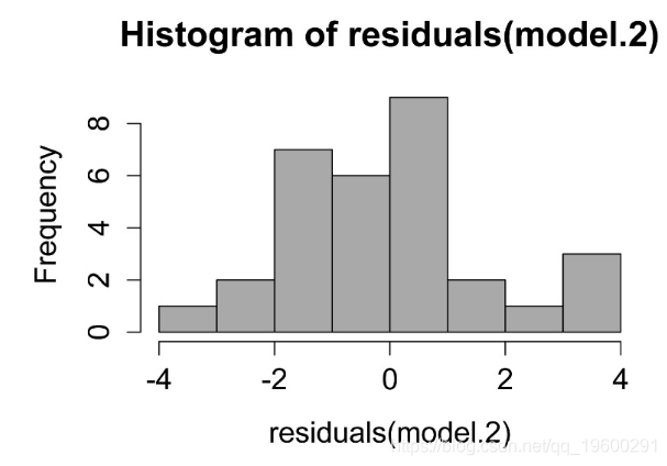
hist(residuals(model.2),
     col="darkgray")
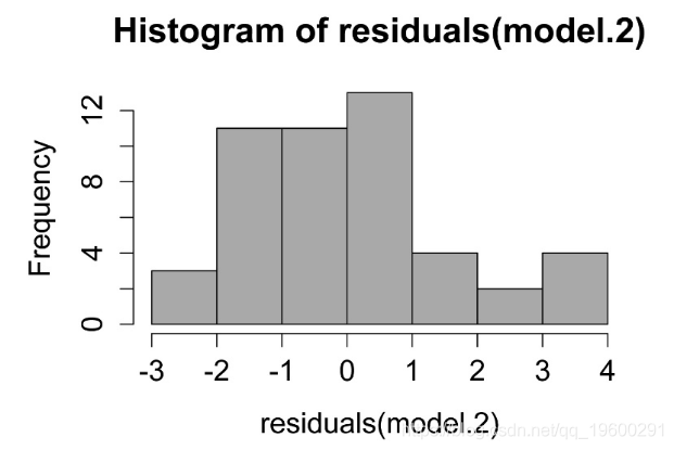
![]() ?
?
线性模型中残差的直方图。这些残差的分布应近似正态。
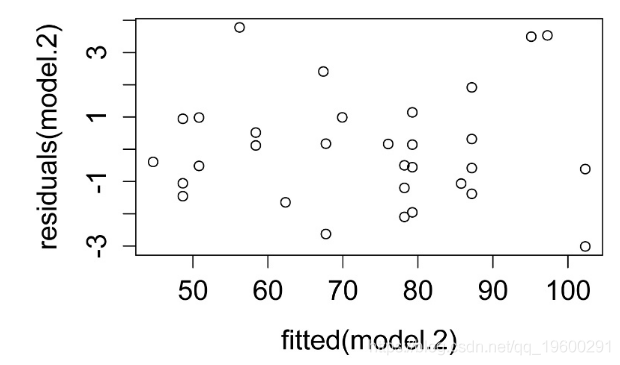
plot(fitted(model.2),
residuals(model.2)) 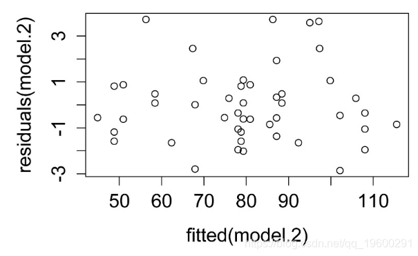
![]() ?
?
残差与预测值的关系图。残差应无偏且均等。
### additional model checking plots with: plot(model.2)
### alternative: library(FSA); residPlot(model.2)
大数据部落 -中国专业的第三方数据服务提供商,提供定制化的一站式数据挖掘和统计分析咨询服务
统计分析和数据挖掘咨询服务:y0.cn/teradat(咨询服务请联系官网客服)
![]() ?
?QQ:3025393450
![]() ?QQ交流群:186388004
?QQ交流群:186388004 
【服务场景】
科研项目; 公司项目外包;线上线下一对一培训;数据爬虫采集;学术研究;报告撰写;市场调查。
【大数据部落】提供定制化的一站式数据挖掘和统计分析咨询


欢迎选修我们的R语言数据分析挖掘必知必会课程!

原文:https://www.cnblogs.com/tecdat/p/12051523.html