tensorflow1.15
scipy
matplotlib (运行时可能会遇到module tkinter的问题)
sklearn 一个基于Python的第三方模块。sklearn库集成了一些常用的机器学习方法。
import matplotlib.pyplot as plt
import numpy as np
import tensorflow as tf
from sklearn import datasets
from tensorflow.python.framework import ops
ops.reset_default_graph()

sess = tf.Session()
Session是tensorflow中的一个执行OP和计算tensor的一个类。
补充:
- 张量(tensor):TensorFlow程序使用tensor数据结构来代表所有的数据,计算图中,操作间传递的数据都是tensor,你可以把TensorFlow tensor看做一个n维的数组或者列表。
- 变量(Variable):常用于定义模型中的参数,是通过不断训练得到的值。比如权重和偏置。
- 占位符(placeholder):输入变量的载体。也可以理解成定义函数时的参数。
- 图中的节点操作(op):一个op获得0个或者多个Tensor,执行计算,产生0个或者多个Tensor。op是描述张量中的运算关系,是网络中真正结构。
# Load the data
# 加载iris数据集并为每类分离目标值。
# 因为我们想绘制结果图,所以只使用花萼长度和花瓣宽度两个特征。
# 为了便于绘图,也会分离x值和y值
# iris.data = [(Sepal Length, Sepal Width, Petal Length, Petal Width)]
iris = datasets.load_iris()
x_vals = np.array([[x[0], x[3]] for x in iris.data])
y_vals1 = np.array([1 if y==0 else -1 for y in iris.target])
y_vals2 = np.array([1 if y==1 else -1 for y in iris.target])
y_vals3 = np.array([1 if y==2 else -1 for y in iris.target])
y_vals = np.array([y_vals1, y_vals2, y_vals3])
#取前两项作为图的横纵坐标
class1_x = [x[0] for i,x in enumerate(x_vals) if iris.target[i]==0]
class1_y = [x[1] for i,x in enumerate(x_vals) if iris.target[i]==0]
class2_x = [x[0] for i,x in enumerate(x_vals) if iris.target[i]==1]
class2_y = [x[1] for i,x in enumerate(x_vals) if iris.target[i]==1]
class3_x = [x[0] for i,x in enumerate(x_vals) if iris.target[i]==2]
class3_y = [x[1] for i,x in enumerate(x_vals) if iris.target[i]==2]
datasets是sklearn中的 一个包,提供了一些经典的数据集以作模型的运算。
特征存储在iris.data中,标签存储在iris.target中
# Declare batch size
# 变量的最高维度
batch_size = 50

# Initialize placeholders
# 数据集的维度在变化,从单类目标分类到三类目标分类。
# 我们将利用矩阵传播和reshape技术一次性计算所有的三类SVM。
# 注意,由于一次性计算所有分类,
# y_target占位符的维度是[3,None],模型变量b初始化大小为[3,batch_size]
x_data = tf.placeholder(shape=[None, 2], dtype=tf.float32)
y_target = tf.placeholder(shape=[3, None], dtype=tf.float32)
prediction_grid = tf.placeholder(shape=[None, 2], dtype=tf.float32)

# Create variables for svm
b = tf.Variable(tf.random_normal(shape=[3,batch_size]))

# Gaussian (RBF) kernel 核函数只依赖x_data
gamma = tf.constant(-10.0)
#dist = tf.reduce_sum(tf.square(x_data), 1)
#dist = tf.reshape(dist, [-1,1])
sq_dists = tf.multiply(2., tf.matmul(x_data, tf.transpose(x_data)))

my_kernel = tf.exp(tf.multiply(gamma, tf.abs(sq_dists)))
tf.placeholder()--占位符相当于预先分配
reduce()--减小矩阵维数,求和
reshape--重新构造矩阵
注:
multiply--实现元素相乘,相同位置的元素相乘
matmul--实现矩阵相乘
Python 矩阵传播--Python为优化矩阵计算的一系列方法
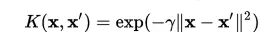
高斯核函数
# Declare function to do reshape/batch multiplication
# 最大的变化是批量矩阵乘法。
# 最终的结果是三维矩阵,并且需要传播矩阵乘法。
# 所以数据矩阵和目标矩阵需要预处理,比如xT·x操作需额外增加一个维度。
# 这里创建一个函数来扩展矩阵维度,然后进行矩阵转置,
# 接着调用TensorFlow的tf.batch_matmul()函数
# 转置后的矩阵与原矩阵相乘(增维可能是为了消除参数项中的常数项)
def reshape_matmul(mat):
  v1 = tf.expand_dims(mat, 1)
  v2 = tf.reshape(v1, [3, batch_size, 1])
  return(tf.matmul(v2, v1))

# Compute SVM Model 计算对偶损失函数
first_term = tf.reduce_sum(b)
b_vec_cross = tf.matmul(tf.transpose(b), b)
y_target_cross = reshape_matmul(y_target)

second_term = tf.reduce_sum(tf.multiply(my_kernel, tf.multiply(b_vec_cross, y_target_cross)),[1,2])
loss = tf.reduce_sum(tf.negative(tf.subtract(first_term, second_term)))
# Gaussian (RBF) prediction kernel
# 现在创建预测核函数。
# 要当心reduce_sum()函数,这里我们并不想聚合三个SVM预测,
# 所以需要通过第二个参数告诉TensorFlow求和哪几个
rA = tf.reshape(tf.reduce_sum(tf.square(x_data), 1),[-1,1])
rB = tf.reshape(tf.reduce_sum(tf.square(prediction_grid), 1),[-1,1])
pred_sq_dist = tf.add(tf.subtract(rA, tf.multiply(2., tf.matmul(x_data, tf.transpose(prediction_grid)))), tf.transpose(rB))
pred_kernel = tf.exp(tf.multiply(gamma, tf.abs(pred_sq_dist)))

# 实现预测核函数后,我们创建预测函数。
# 与二类不同的是,不再对模型输出进行sign()运算。
# 因为这里实现的是一对多方法,所以预测值是分类器有最大返回值的类别。
# 使用TensorFlow的内建函数argmax()来实现该功能
prediction_output = tf.matmul(tf.multiply(y_target,b), pred_kernel)
prediction = tf.arg_max(prediction_output-tf.expand_dims(tf.reduce_mean(prediction_output,1), 1), 0)
accuracy = tf.reduce_mean(tf.cast(tf.equal(prediction, tf.argmax(y_target,0)), tf.float32))

# Declare optimizer
my_opt = tf.train.GradientDescentOptimizer(0.01)
train_step = my_opt.minimize(loss)

# Initialize variables
init = tf.global_variables_initializer()
sess.run(init)
# Save graph
write_log = tf.summary.FileWriter(‘./log‘,tf.get_default_graph())

# Training loop
loss_vec = []
batch_accuracy = []
for i in range(100):
  #取随机数训练模型
  rand_index = np.random.choice(len(x_vals), size=batch_size)
  rand_x = x_vals[rand_index]
  rand_y = y_vals[:,rand_index]
  sess.run(train_step, feed_dict={x_data: rand_x, y_target: rand_y})

  temp_loss = sess.run(loss, feed_dict={x_data: rand_x, y_target: rand_y})
  loss_vec.append(temp_loss)

  acc_temp = sess.run(accuracy, feed_dict={x_data: rand_x,
                       y_target: rand_y,
                       prediction_grid:rand_x})
  batch_accuracy.append(acc_temp)

  if (i+1)%25==0:
    print(‘Step #‘ + str(i+1))
    print(‘Loss = ‘ + str(temp_loss))

# 创建数据点的预测网格,运行预测函数
x_min, x_max = x_vals[:, 0].min() - 1, x_vals[:, 0].max() + 1
y_min, y_max = x_vals[:, 1].min() - 1, x_vals[:, 1].max() + 1
xx, yy = np.meshgrid(np.arange(x_min, x_max, 0.02),
           np.arange(y_min, y_max, 0.02))
grid_points = np.c_[xx.ravel(), yy.ravel()]
grid_predictions = sess.run(prediction, feed_dict={x_data: rand_x,
                          y_target: rand_y,
                          prediction_grid: grid_points})
grid_predictions = grid_predictions.reshape(xx.shape)
# 测试random.choice程序
import numpy as np
x=np.array([[0,1],[1,2],[2,3]])
randx=np.random.choice(len(x), size=3)
print(x)
#print(‘\n‘)
print(randx)
print(x[randx])
#print(x[:,randx])
print(len(x))

原文:https://www.cnblogs.com/speakdaliy/p/12085309.html