Node Embeddings
Map nodes to low-dimensional embeddings.
Goal, \(similarity(u, v) \approx z_u ^Tz_v\) is to encode nodes so that similarity in the embedding space approximates similarity in the original network.
Two Key Components
- Encoder maps each node to a low-dimensional vector.
- Similarity function specifies how relationships in embedding space map to relationships in the original network.
From "Shallow" to "Deep"
shallow encoders, i.e. One-hot encoder
Limitations of shallow encoding:
- \(O(\vert V \vert )\) parameters are needed: there is no parameter sharing and every node has its own unique embedding vector.
- Inherently "transductive": It is impossible to generate embeddings for nodes that were not seen during training.
- Do not incorporate node features: Many graphs have features that we can and should leverage.
We will now discuss "deeper" methods based on graph neural networks. \(ENC(v)\) function is a complex function that depends on graph structure. In general, all of these more complex encoders can be combined with the similarity functions.
The Basics: Graph Neural Networks
Setup
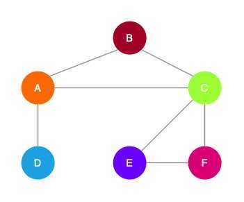
Assume we have a graph \(G\):
- \(V\) is the vertex set.
- \(A\) is the adjacency matrix (assume binary).
- \(X \in R ^{m \times \vert V \vert}\) is a matrix of node features.
- Categorical attributes, text, image data, e.g., profile information in a social network.
- Node degrees, clustering coefficients, etc.
- Indicator vectors (i.e., one-hot encoding of each node).
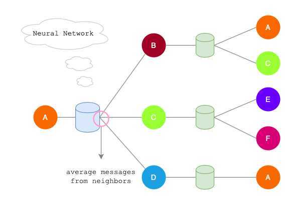
Neighborhood Aggregation
Key idea: Generate node embeddings based on local neighborhoods.
Intuition
- Nodes aggregate information from their neighbors using neural networks.
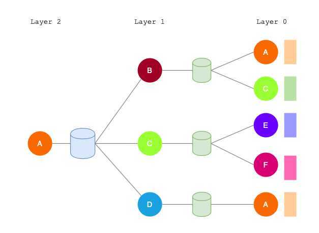
- Network neighborhood defines a computation graph.
- Every node defines a unique computation graph.
- Nodes have embeddings at each layer.
- Model can be arbitrary depth.
- "layer-0" embedding of node \(u\) is its input feature, i.e. \(x_u\).
Neighborhood aggregation can be viewed as a center-surround filter.
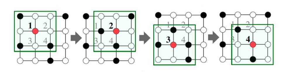
Neighborhood aggregation mathematically related to spectral graph convolutions.
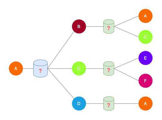
Key distinctions are in how different approaches(the boxes between layers) aggregate information across the layers.
Methods
Basic approach:
Average neighbor information and apply a neural network.
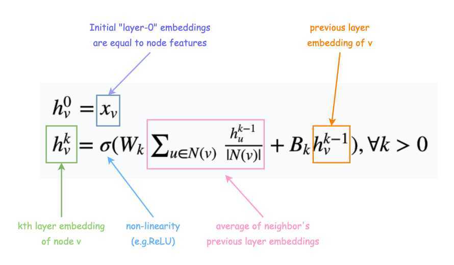
Math: Expression (1)
\(h_v^0 = x_v\)
\(h_v^k = \sigma (W_k \sum _{u \in N(v)} \frac{h_u^{k-1}}{\vert N(v) \vert } + B_k h_v^{k-1}), \forall k > 0\)
Traning the Model
What we should learn?
- In Expression (1), \(W_k, B_k\) are the trainable matrices
- After K-layers of neighborhood aggregation, we get output embeddings for each node.
Loss function
- We can feed these embeddings into any loss function and run stochastic gradient descent to train the aggregation parameters.
- Train in an unsupervised manner using only the graph structure.
- Unsupervised loss function can be based on
- Random walks (node2vec, DeepWalk)
- Graph factorization
Alternative
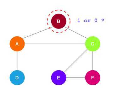
- Directly train the model for a supervised task (e.g., node classification)
Overview of Model Design
- Define a neighborhood aggregation function, i.e. neural network.
- Define a loss function on the embeddings, \(L(z_u)\).
- Train on a set of nodes, i.e., a batch of compute graphs. Note that not all nodes are used for training!
- Generate embeddings for all nodes (Even for nodes we never trained on).
Inductive Capability
- The same aggregation parameters are shared for all nodes.
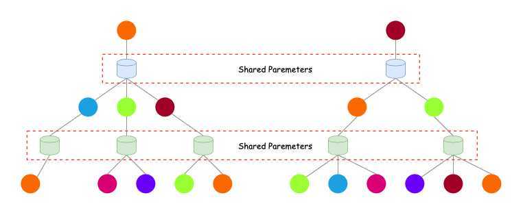
- The number of model parameters is sublinear in $\vert V \vert $ and we can generalize to unseen nodes.
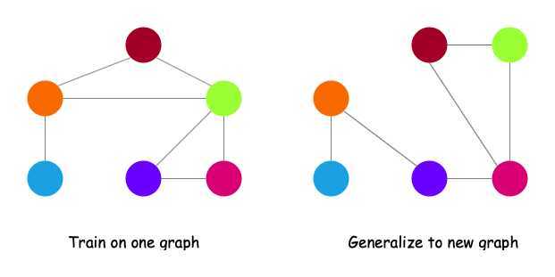
- Inductive node embedding \(\Rightarrow\) generalize to entirely unseen graphs, e.g., train on protein interaction graph from model organism A and generate embeddings on newly collected data about organism B
An Introduction on Graph Neural Network
原文:https://www.cnblogs.com/luyunan/p/12423728.html