Scheduling
- Workload Assumptions
? First, we want to understand the scheduling that we must know what to schedule. Therefore, we will make a number of simplifying assumptions about processes running in the system, called workload. Here are details about workload:
- Run time
- Arrive time
- Complete time
Using these assumptions, we can judge a scheduling by some metrics.
- Scheduling metrics
- Turnaround time
We can define the turnaround time as:
\(T_{turnaround} = T_{completion} - T_{arrival}\)
- Response time
We can define the Response time as:
\(T_{response} = T_{fisrturn} - T_{arrival}\)
Since we have the metrics that can judge the quality of scheduling, let‘s see some traditional scheduling.
- First in, First out(FIFO)
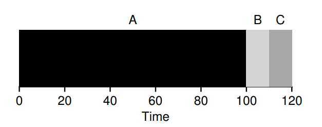
? This scheduling, like traditional Queue, is a simply scheduling. But, suppose lots of jobs arrival simultaneously, if a job has long-time run time first, the lefts must wait it. Therefore, the \(T_{turnaround}\) and \(T_{response}\) are longer than short-time job run first. It is not a better scheduling in modorn system.


Shorest Job First(SJF)
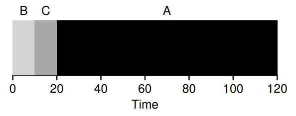
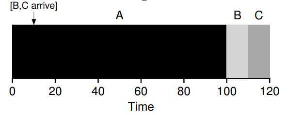
? The scheduling are propose to solve above FIFO. Due to run the short-time job first, it guarantee short-time job will not wait for long-time task. So the \(T_{turnaround}\) will be improved, but still remain two quesition: First, the \(T_{response}\) will be not improved. Second, how to deal with if jobs not arrival simultaneously?


Shortest Time-to-completion First(STCF)
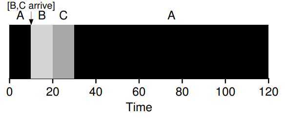
? The scheduling will solve the quesition if jobs arrival asynchronous. It bases on a notion called preempt, which let the scheduling to determine which of remaining jobs has the least time left, and schedules that one. The scheduling will make the \(T_{turnaround}\) almost perfect, but \(T_{response}\) still badly.

Round Robin(RR)
? The scheduling will improve the \(T_{response}\). Also, it bases on a notion called time slice(sometimes called a scheduling quantum). It schedules a job running for a time slice and then switching to the next job in the run queue, repeatedly does so until all jobs are finished. Deviously, the key point of the scheduling is the length of time slice. The shorter it is, the better performance of RR under the response-time metrics. However, making time slice too short is problematic: suddenly the cost of context switching will dominate overall performance. Thus, deciding on the length of time slice presents a trade-off to a system designer, making it long enough to amortize the cost of switching without making it so long that system is no longer response. (Note that the cost of context switching does not arise solely from the OS actions of saving and restoring a few registers. When programs run, they build up a great deal of state in CPU caches, TLBs, branch predictors, and other on-chip hardware. Switching to another job causes this state to be flushed and new state relevant to the currently-running job to be brought in, which may exact a noticeable performance cost)

? For example, if the time slice is set of \(10ms\), and the switching cost is \(1ms\), roughly \(10%\) of time is spent context switching and is thus wasted. If we want to amortize this cost, we can increase the time slice, e.g., to \(100ms\). In this case, less than \(1%\) of time is spent context switching, and thus the cost of time slice has been amortized.
incorporating I/O using overlap
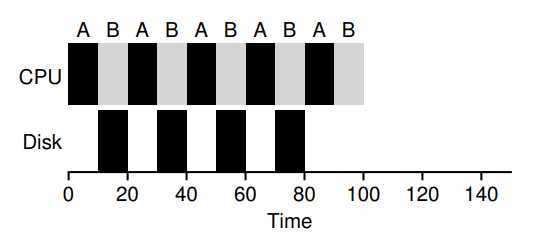
? A scheduler clearly has a decision to make when a jog initiates an I/O request, because the currently-running job won‘t be using the CPU during I/O, it is blocked waiting for I/O completion. If I/O sent a hard-disk drive, the process will be blocked few ms or longer. Thus, the scheduler should probably schedule another job on CPU at that time.
? The scheduler also has a decision to make when the I/O completes. When that occurs, an interrupt is raised, and the OS runs and moves the process that issued I/O from blocked to ready state.
? To better use the CPU‘s resources, we can use STCF.

After study above, we know that \(T_{turnaround}\) and \(T_{response}\) like a coin(once can only satisfy one side). More generally, any policy(such as RR) that is fair, that evenly divides the CPU among active processes on a small time slice, will perform poorly on metrics such as turnaround time. Indeed, this is an inherent trade-off: if you are willing to be unfair, if you are willing to be unfair, you can run shorter jobs to completion, but at the cost of response time; if you instead value fairness, response time is lowered, but at the cost of turnaround time. This type of trade-off is common in systems.
We have developed two types of schedulers. The first type (SJF, STCF) optimizes turnaround time, but is bad for response time. The second type (RR) optimizes response time but is bad for turnaround. However, the first type based on the precisely time a job will run, for many real jobs it is unrealistic. Therefore, we must find a scheduler that do not know real time and still run effectively, moreover, if can balance between turnaround time and response time be better.
- Multi-level feedback queue (MLFQ)
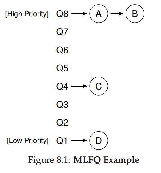
? Because we don‘t know the precise time a job would run, we only know the job‘s history. In statistic, the history is important notion that can predict the future. Based on it, we also can learn from job‘s history to judge its behavour, these style scheduler, we called MLFQ. The MLFQ has a number of distinct queues, each assigned a different priority level. At any given time, a job that is ready to run is on a single queue. MLFQ uses priorities to decide which job should run at a given time: a job with higher priority (i.e, a job on higher queue) is chosen to run, if more than one job may be in given queue, and thus have same priority, in this case, we will just use round-robin scheduling among these jobs.

So, we can give some policy about MLFQ that can make us understand readily.
- Ruler 1: If Priority(A) > Priority(B), A runs (B doesn‘t).
- Ruler 2: If Priority(A) = Priority(B), A & B run in RR.
? The MLFQ is based on priority, so how do we change jobs‘ priority? To do this, we must keep in mind our workload: a mix of interactive jobs that are short-running (and may frequently relinquish the CPU), and some longer-running “CPU-bound” jobs that need a lot of CPU time but where response time isn’t important.
Due to learn from history, we can suppose a job are short-running-time and change its priority based on its behavour.
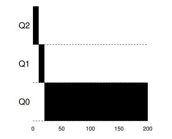
- Ruler 3: When a job enters the system, it is placed at the highest priority (the topmost queue).
- Ruler 4a: If a job uses up an entire time slice while running, its priority is reduced (i.e., it moves down one queue).
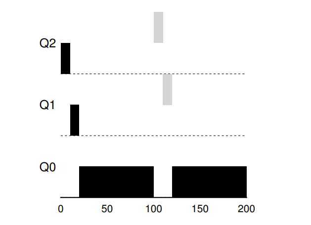
- Ruler 4b: If a job gives up the CPU before the time slice is up, it stays at the same priority level.
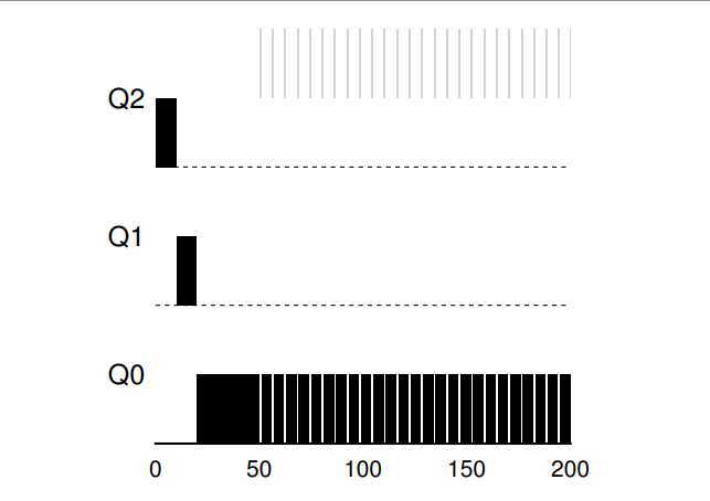
There are three example you can see:
A single long-running job. Along came A short job. Some job with I/O.


? The current MLFQ seems to do fairness job, sharing CPU fairly. Unfortunately, the scheduler we have developed thus far contains serious flaws.
? First, if a long-running job have runned and reduced to lower queue, then some of I/O frequently job (interactive job) arrive. What happen? Deviously, the long-running job will be starvation, that is, interactive jobs will combine to assume all CPU time, and thus long-running jobs will never receive any CPU time (they starve).
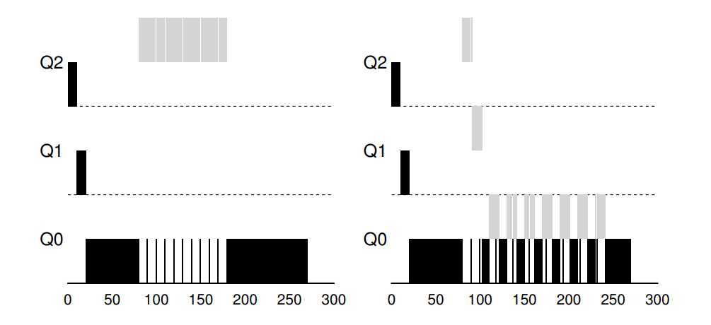
? Second, a smarter user could rewrite program to game the scheduler, Gaming the scheduler generally refers to the idea of doing something sneaky to trick the scheduler into giving you more than your fair share of the resource. The algorithm we have described is susceptible to the following attack: before the time slice is over, issue an I/O operation (to some file you don’t care about) and thus relinquish the CPU; doing so allows you to remain in the same queue, and thus gain a higher percentage of CPU time. When done right (e.g., by running for 99% of a time slice before relinquishing the CPU), a job could nearly monopolize the CPU.
? Third, a job may change its behaviour over time; what was CPU-bound may transition to a phase of interactivity. With our current approach, such a job would be out of luck and not be treated like the other interactive jobs in the system.
- The priority boost
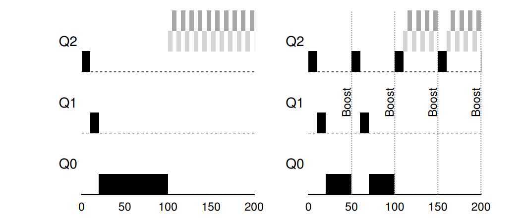
? To solve the first and third problem, we can periodically boost the priority of all jobs in system. There are many ways to achieve this, but let‘s just do something simple: throw them all in the topmost queue; hence, a new ruler:
- Ruler 5: After some time period S, move all jobs in the system to topmost queue.
? First, processes are guaranteed not to starve: by sitting in the top queue, a job will share the CPU with other high-priority jobs in RR-fashion, and eventually receive server. Third, if a CPU-bound job has become interactive, the scheduler treats it properly once it has received the priority boost.

? Due to the second problem based on time slice and I/O, so we can perform better accounting of CPU time at each level of the MLFQ. Instead of forgetting how much of a time slice a process used at a given level, the scheduler should keep track. Once a process has used its allotment, it is demoted to the next priority queue. Whether it uses the time slice in on long burst or many small ones does not matter. We thus rewrite Ruler 4a and 4b as:
Ruler 4: Once a job uses up its time allotment at a given level (regardless of how many times it has given up the CPU), its priority is reduced.

Parameterize MLFQ
? There are many parameter in MLFQ, such as boost period time S, length of time slice, or the time of per-level allotment. The MLFQ‘s performance depends on these parameters, so how do we set it?
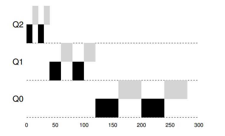
? For example, most MLFQ variants allow for varying time-slice length across different queues. The high-priority queues are usually given short time slices; they are comprised of interactive jobs, after all, and thus quickly alternating between them makes sense. The low-priority queues, in contrast, contain long-running jobs that are CPU-bound; hence, longer time slices work well.

Different MLFQs have different features, we do not talk more about them. We can see man page of them to see details.
- Proportional Share
? Contrast with schedulers above, we will examine a different type of scheduler known as a proportional-share scheduler, also sometimes referred to as a fair-share scheduler.
- lottery scheduling
? Although the idea is certainly older, it still have value that we have to learn. The basic idea is quite simple: every so often, hold a lottery to determine which process should get to run next; processes that should run more often should be given more chances to win the lottery.
- Tickets represent your share
? The tickets are used to represent the share of a resource that a process should receive. For example, there are two processes, A and B, process A has \(75\) tickets while B only has \(25\). Thus, what we would like is for A to receive \(75\%\) of the CPU and B the remaining \(25\%\).
? Lottery scheduling achieves this probabilistically (but not deterministically) by holding a lottery every so often (say, every time slice). Holding a lottery is straightforward: the scheduler must know how many total tickets there are (in out example, there are 100). The scheduler then picks a winning ticket, which is a number from 0 to 99. Assuming A holds tickets 0 through 74 and B 75 through 99, the winning ticket simply determines whether A or B wins.
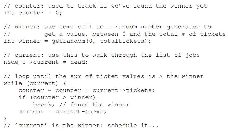
? How to implementation the scheduling? Not only do the notion are simply, but the implementation also, it just uses a normally List, let me show you the pseudocode to understand intuitive.

An example
? To make the dynamics of lottery scheduling more understandable, we now perform a brief study of the completion time of two jobs competing against one another, each with the same number of tickets (100) and same run time (\(R\), which we will vary).
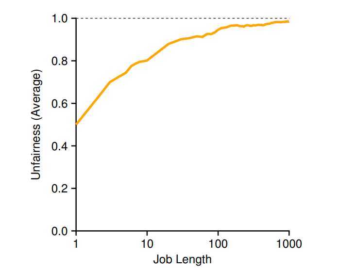
? In this scenario, we’d like for each job to finish at roughly the same time, but due to the randomness of lottery scheduling, sometimes one job finishes before the other. To quantify this difference, we define a simple unfairness metric, \(U\) which is simply the time the first job completes divided by the time that the second job completes. For example, if \(R = 10\), and the first job finishes at time 10 (and the second job at 20), \(U = 10/20 = 0.5\). When both jobs finish at nearly the same time, \(U\) will be quite close to 1. In this scenario, that is our goal: a perfectly fair scheduler would achieve \(U\) = 1.
? Figure plots the average unfairness as the length of the two jobs (\(R\)) is varied from 1 to 1000 over thirty trials (results are generated via the simulator provided at the end of the chapter). As you can see from the graph, when the job length is not very long, average unfairness can be quite severe. Only as the jobs run for a significant number of time slices does the lottery scheduler approach the desired outcome. (Law-of-large-numbers)

- Ticket mechanisms
? Lottery scheduling also provides a number of machanisms to manipulate tickets in different and somethings useful ways.
- ticket currency
? Currency allows a user with a set of tickets to allocate tickets among their own jobs in whatever currency they would like; the system then automatically converts said currency into the correct global value. For example, assume users A and B have each been given 100 tickets. User A is running two jobs, A1 and A2, and gives them each 500 tickets (out of 1000 total) in User A’s own currency. User B is running only 1 job and gives it 10 tickets (out of 10 total). The system will convert A1’s and A2’s allocation from 500 each in A’s currency to 50 each in the global currency; similarly, B1’s 10 tickets will be converted to 100 tickets. The lottery will then be held over the global ticket currency (200 total) to determine which job runs.
- ticket transfer
? With transfer, a process can temporarily hand off its tickets to another process. This ability is especially useful in a client/server setting, where a client process sends a message to a server asking it to do some work on client‘s behalf. To speed up the work, the client can pass tickets to the server and thus try to maximize the performance of the server while the server is handling the client‘s request. When finished, the server then transfers the tickets back to the client and all is as before.
- ticket inflation
? With ticket inflation, a process can temporarily raise or lower the number of tickets it owns. Of cource, in a competitive scenario with processes that do not trust one another, this makes little sense; one greedy process could give itself a vast number of tickets and take over the machine. Rather, inflation can be applied in an environment where a group of processes trust one another; in such a case, if any one process knows it need more CPU resource, it can boost its tickets value as a way to reflect that need to the system, all without communicating with any other processes.
Like the MLFQ above, how to assign the tickets is important about the scheduling. One approach is to assume that users know best; in such a case, each user is handed some number of tickets, and a user can allocate tickets to any jobs they run as desired. However, this solution is a non-solution: it really doesn‘t tell you what to do. Thus, give a set of jobs, the problem remains open.
- Why not deterministic?
? Why we use randomness at all? As we saw above, while randomness gets us simple scheduler, it occasionally will not deliver the exact right proportions, especially over short time scales. For this reason, the stride scheduling, a deterministic fair-share scheduler, is proposed.
? Stride scheduling is also straightforward. Each job in the system has a stride, which is inverse in proportion to the number of tickets it has. In our example above, with jobs A, B, and C, with 100, 50, and 250 tickets, respectively, we can compute the stride of each by dividing some large number by the number of tickets each process has been assigned. For example, if we divide 10,000 by each of those ticket values, we obtain the following stride values for A, B, and C: 100, 200, and 40. We call this value the stride of each process; every time a process runs, we will increment a counter for it (called its pass value) by its stride to track its global progress.
? The scheduler then uses the stride and pass to determine which pro?cess should run next. The basic idea is simple: at any given time, pick the process to run that has the lowest pass value so far; when you run a process, increment its pass counter by its stride. A pseudocode will understandable.

? So you might be wondering: given the precision of stride scheduling, why use lottery scheduling at all? Well, lottery scheduling has one nice property that stride scheduling does not: no global state. Imagine a new job enters in the middle of our stride scheduling example above; what should its pass value be? Should it be set to 0? If so, it will monopolize the CPU. With lottery scheduling, there is no global state per process; we simply add a new process with whatever tickets it has, update the single global variable to track how many total tickets we have, and go from there. In this way, lottery makes it much easier to incorporate new processes in a sensible manner.
- The Linux Completely Fair Scheduler(CFS)
? Despite these earlier works in fair-share scheduling, the current Linux approach achieves similar goals in an alternate manner. The scheduler, entitled the Completely Fair Scheduler (or CFS), implements fair-share scheduling, but does so in a highly efficient and scalable manner.
? To achieve its efficiency goals, CFS aims to spend very little time mak?ing scheduling decisions, through both its inherent design and its clever use of data structures well-suited to the task. Recent studies have shown that scheduler efficiency is surprisingly important; specifically, in a study of Google datacenters, Kanev et al. show that even after aggressive optimization, scheduling uses about 5% of overall datacenter CPU time. Re?ducing that overhead as much as possible is thus a key goal in modern scheduler architecture.
- Basic Operation
? Whereas most schedulers are based around the concept of a fixed time slice, CFS operates a bit differently. (Like RR-fasion or lottery scheduler) Its goal is simple: to fairly divide a CPU evenly among all competing processes. It does so through a simple counting-based technique known as virtual runtime (vruntime).
? As each process runs, it accumulates vruntime. In the most basic case, each process’s vruntime increases at the same rate, in proportion with physical (real) time. When a scheduling decision occurs, CFS will pick the process with the lowest vruntime to run next.
? a
Operating system Chapter 7-9
原文:https://www.cnblogs.com/GRedComeT/p/12459409.html

