转载自:https://www.cnblogs.com/php-rearch/p/6760683.html
前言
今天群里有人问到一个图像的问题,但本质上是一个基本最小二乘问题,涉及到霍夫变换(Hough Transform),用到了就顺便总结一下。
内容为自己的学习记录,其中多有参考他人,最后一并给出链接。
一、霍夫变换(Hough)
A-基本原理
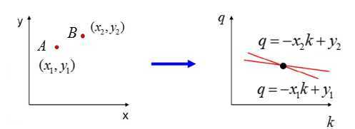
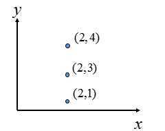
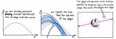
一条直线可由两个点A=(X1,Y1)和B=(X2,Y2)确定(笛卡尔坐标)
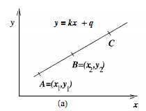
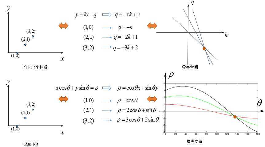
另一方面, 也可以写成关于(k,q)的函数表达式(霍夫空间):
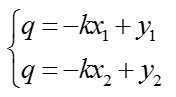
对应的变换可以通过图形直观表示:
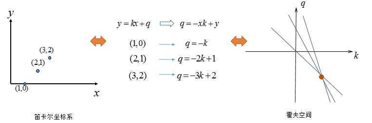
变换后的空间成为霍夫空间。即:笛卡尔坐标系中一条直线,对应霍夫空间的一个点。
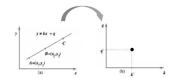
反过来同样成立(霍夫空间的一条直线,对应笛卡尔坐标系的一个点):
再来看看A、B两个点,对应霍夫空间的情形:
一步步来,再看一下三个点共线的情况:
可以看出如果笛卡尔坐标系的点共线,这些点在霍夫空间对应的直线交于一点:这也是必然,共线只有一种取值可能。
如果不止一条直线呢?再看看多个点的情况(有两条直线):
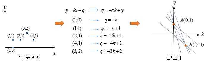
其实(3,2)与(4,1)也可以组成直线,只不过它有两个点确定,而图中A、B两点是由三条直线汇成,这也是霍夫变换的后处理的基本方式:选择由尽可能多直线汇成的点。
看看,霍夫空间:选择由三条交汇直线确定的点(中间图),对应的笛卡尔坐标系的直线(右图)。
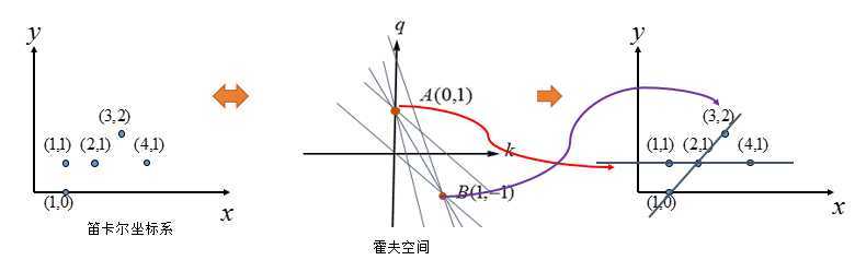
到这里问题似乎解决了,已经完成了霍夫变换的求解,但是如果像下图这种情况呢?
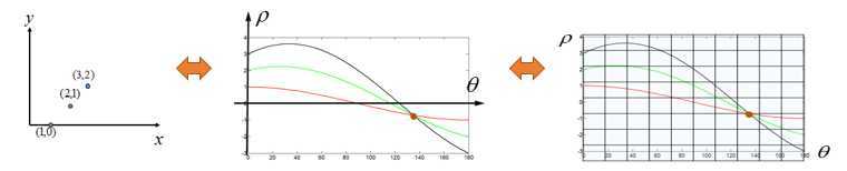
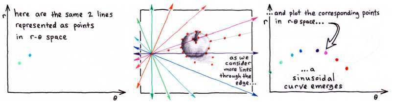
k=∞是不方便表示的,而且q怎么取值呢,这样不是办法。因此考虑将笛卡尔坐标系换为:极坐标表示。
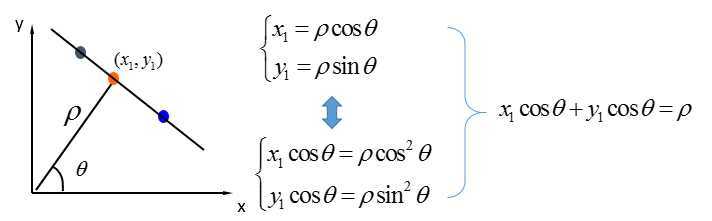
在极坐标系下,其实是一样的:极坐标的点→霍夫空间的直线,只不过霍夫空间不再是[k,q]的参数,而是![]() 的参数,给出对比图:
的参数,给出对比图:
是不是就一目了然了?
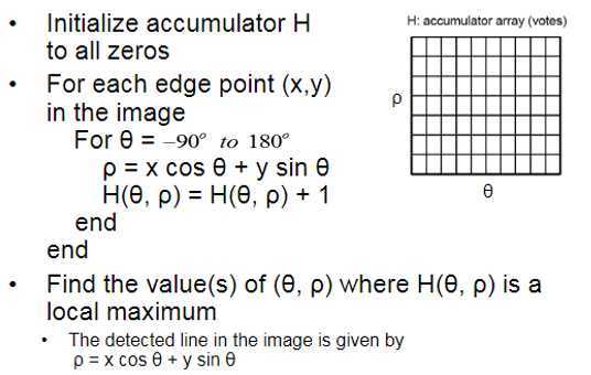
给出霍夫变换的算法步骤:
对应code:
|
1
2
3
4
5
6
7
8
9
10
11
12
13
14
15
16
17
18
19
20
21
22
23
24
25
|
function [ Hough, theta_range, rho_range ] = naiveHough(I)%NAIVEHOUGH Peforms the Hough transform in a straightforward way.%[rows, cols] = size(I);theta_maximum = 90;rho_maximum = floor(sqrt(rows^2 + cols^2)) - 1;theta_range = -theta_maximum:theta_maximum - 1;rho_range = -rho_maximum:rho_maximum;Hough = zeros(length(rho_range), length(theta_range));for row = 1:rows for col = 1:cols if I(row, col) > 0 %only find: pixel > 0 x = col - 1; y = row - 1; for theta = theta_range rho = round((x * cosd(theta)) + (y * sind(theta))); %approximate rho_index = rho + rho_maximum + 1; theta_index = theta + theta_maximum + 1; Hough(rho_index, theta_index) = Hough(rho_index, theta_index) + 1; end end endend |
其实本质上就是:
交点怎么求解呢?细化成坐标形式,取整后将交点对应的坐标进行累加,最后找到数值最大的点就是求解的![]() ,也就求解出了直线。
,也就求解出了直线。
B-理论应用
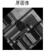
这里给出MATLAB自带的一个应用,主要是对一幅图像进行直线检验,原图像为:
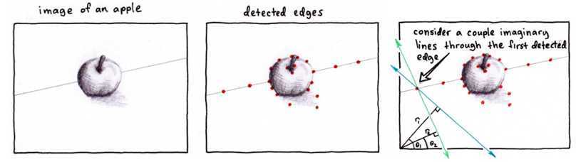
首先是对其进行边缘检测:
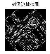
边缘检测后并二值化,就可以通过找非零点的坐标确定数据点。从而对数据点进行霍夫变换。对应映射到霍夫空间的结果为:
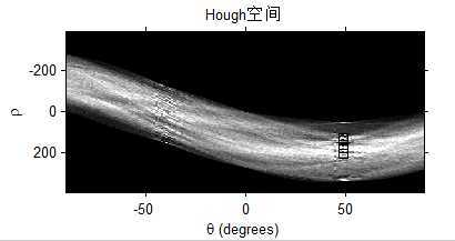
找出其中数值较大的一些点,通常可以给定一个阈值,Threshold一下。
这就完成了霍夫变换的整个过程。这个时候求解出来了其实就是多条直线的斜率k以及截距q,通常会根据直线的特性进一步判断,从而将直线变为线段:
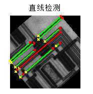
不过这一步更类似后处理,其实已经不是霍夫变换本身的特性了。
给出对应的代码:
|
1
2
3
4
5
6
7
8
9
10
11
12
13
14
15
16
17
18
19
20
21
22
23
24
25
26
27
28
29
30
31
32
33
34
35
36
37
38
39
40
41
42
43
44
|
clc;clear all;close all;I = imread(‘circuit.tif‘);rotI = imrotate(I,40,‘crop‘);subplot 221fig1 = imshow(rotI);BW = edge(rotI,‘canny‘);title(‘原图像‘);subplot 222imshow(BW);[H,theta,rho] = hough(BW);title(‘图像边缘检测‘);subplot 223imshow(imadjust(mat2gray(H)),[],‘XData‘,theta,‘YData‘,rho,... ‘InitialMagnification‘,‘fit‘);xlabel(‘\theta (degrees)‘), ylabel(‘\rho‘);axis on, axis normal, hold on;colormap(hot)P = houghpeaks(H,5,‘threshold‘,ceil(0.7*max(H(:))));x = theta(P(:,2));y = rho(P(:,1));plot(x,y,‘s‘,‘color‘,‘black‘);lines = houghlines(BW,theta,rho,P,‘FillGap‘,5,‘MinLength‘,7);title(‘Hough空间‘);subplot 224, imshow(rotI), hold onmax_len = 0;for k = 1:length(lines) xy = [lines(k).point1; lines(k).point2]; plot(xy(:,1),xy(:,2),‘LineWidth‘,2,‘Color‘,‘green‘); % Plot beginnings and ends of lines plot(xy(1,1),xy(1,2),‘x‘,‘LineWidth‘,2,‘Color‘,‘yellow‘); plot(xy(2,1),xy(2,2),‘x‘,‘LineWidth‘,2,‘Color‘,‘red‘); % Determine the endpoints of the longest line segment len = norm(lines(k).point1 - lines(k).point2); if ( len > max_len) max_len = len; xy_long = xy; endend% highlight the longest line segmentplot(xy_long(:,1),xy_long(:,2),‘LineWidth‘,2,‘Color‘,‘red‘);title(‘直线检测‘); |
对比自带的Hough与编写的Hough:
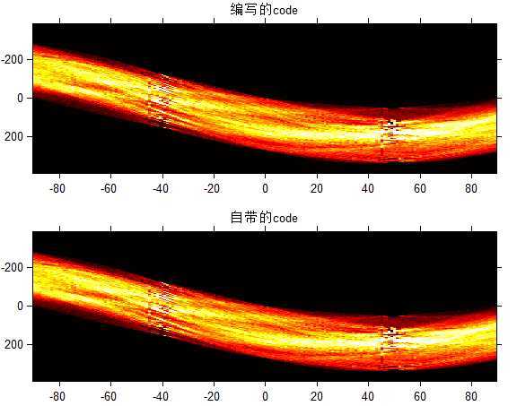
效果还是比较接近的。
看到Stackoverflow上的一个答案,觉得很好,收藏一下:
原文:https://www.cnblogs.com/xuhongfei0021/p/12492130.html