推荐系统系列之三：深度学习家族

1. MLP

来源出处：

• He, Xiangnan, et al. "Neural collaborative filtering." Proceedings of the 26th international conference on world wide web. 2017.

目标函数：

其中，\(\mathbf{O}\) 表示用户 \(u\) 和商品 $i $ 之间有交互记录的集合，其中 \(y_{u,i}=1\) ，\(\mathbf{O^-}\) 表示用户 \(u\) 和商品 $j $ 之间没有交互记录的集合，其中 \(y_{u,j}=0\) 。

说明介绍：

采用神经网络的方法，用交叉熵损失函数对隐式数据进行建模。

核心代码：

def inference(self, users_inputs, items_inputs):
        embed_users = tf.nn.embedding_lookup(
            self.weights[‘embedding_users‘], users_inputs)
        embed_items = tf.nn.embedding_lookup(
            self.weights[‘embedding_items‘],items_inputs)
        layer0 = tf.nn.relu(tf.matmul(tf.concat([embed_items,embed_users],1), 
                      self.weights[‘weight_0‘]) + self.weights[‘bias_0‘])
        layer1 = tf.nn.relu(
            tf.matmul(layer0, self.weights[‘weight_1‘]) + self.weights[‘bias_1‘])       
        y_ = tf.matmul(layer1,self.weights[‘weight_n‘]) + self.weights[‘bias_n‘]
        return y_ 

实验结果：

• 原论文中的实验处理

数据集：Movielens100K，留一评估（leave-one-out）

• 传统随机分割

数据集：Movielens100K，随机分割成训练集：测试集 = 8:2

loss 和 RMSE 的收敛曲线如下图所示：

数据集随机分割这个实验中，本人怎么调参都无法将排序指标（Recall 和 NDCG）提升太多，始终在0.1之下。若谁调出个好结果，望留言告知，谢谢！

对比

• 矩阵分解 MF 实验结果

在关键参数相同的情况下，对比 MF，可以看出其实 MLP 的实验并没提升多少。我想，这也许是原论文作者采用隐式数据加采样训练和留一评估的原因的吧。

2. LSTM

来源出处：

• Wu, Chao-Yuan, et al. "Recurrent recommender networks." Proceedings of the tenth ACM international conference on web search and data mining. 2017.

目标函数：

其中，\(R\left( \theta \right)\) 为正则项。\(u_i\) 和 \(m_j\) 分别表示用户 \(i\) 和电影 \(j\) 的静态属性，\(\tilde{u}_{i,t}\) 和 \(\tilde{m}_{j,t}\) 分别表示他们来自 LSTM 的动态特征向量。

说明介绍：

通过分别对用户和商品得到时间序列进行建模，来获得它们的动态轨迹，然后用它们的动态特征向量来预测评分。

3. Item2vec

来源出处：

• Barkan, Oren, and Noam Koenigstein. "Item2vec: neural item embedding for collaborative filtering." 2016 IEEE 26th International Workshop on Machine Learning for Signal Processing (MLSP). IEEE, 2016.

说明介绍：

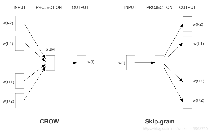
作者将 Word2vec 的思想用到推荐中，Word2vec 输入的是词序列，Item2vec 输入的是 购买的商品序列。

核心代码：

直接参考 Word2vec 代码，数据处理好后，直接在 python 中调用 gensim 包中的 word2vec 函数，然后调参就可以。

4. AutoRec

来源出处：

• Sedhain, Suvash, et al. "Autorec: Autoencoders meet collaborative filtering." Proceedings of the 24th international conference on World Wide Web. 2015.

目标函数：

• Item-based AutoRec：

其中，\(\mathbf{r}_{\cdot,i}\) 表示商品 \(i\) 的所有评分，\(h\left(\mathbf{r}_{\cdot,i},\theta \right)\) 表示模型预测值，\(\mathbf{W}\) 和 \(\mathbf{V}\) 表示自编码器的权重。

• User-based AutoRec：

其中，\(\mathbf{r}_{u,\cdot}\) 表示用户 \(u\) 的所有评分。

说明介绍：

这篇文章采用自编码的方式来预测评分。

核心代码：

# 网络的前向传播
def inference(self, rating_inputs):
    encoder = tf.nn.sigmoid(tf.matmul(rating_inputs, self.weights[‘V‘]) + self.weights[‘mu‘])
    decoder = tf.identity(tf.matmul(encoder, self.weights[‘W‘]) + self.weights[‘b‘])
    return decoder         


def loss_function(self, true_r, predicted_r, lamda_regularizer=1e-3):
    idx = tf.where(true_r>0)
    true_y = tf.gather_nd(true_r, idx)
    predicted_y = tf.gather_nd(predicted_r, idx)
    mse = tf.compat.v1.losses.mean_squared_error(true_y, predicted_y)
    regularizer = tf.contrib.layers.l2_regularizer(lamda_regularizer)
    regularization = regularizer(self.weights[‘V‘]) + regularizer(self.weights[‘W‘])
    cost = mse + regularization
    return cost 

实验结果：

数据集：Movielens100K，随机分割成训练集：测试集 = 8:2

• User-based AutoRec：

• Item-based AutoRec：

5. CDAE (Collaborative Denoising Auto-Encoders)

来源出处：

• Wu, Yao, et al. "Collaborative denoising auto-encoders for top-n recommender systems." Proceedings of the Ninth ACM International Conference on Web Search and Data Mining. 2016.

目标函数：

其中，\(\widetilde{\mathbf{y}}_u\) 和 \(\widehat{\mathbf{y}}_u\) 分别表示网络的输出和输出，\(\mathbf{y}_u\) 表示用户 \(u\) 的所有评分记录，\(\widetilde{\mathbf{y}}_u\) 为 \(\mathbf{y}_u\) 以概率 \(p\) 的 dropout 得到的采样。\(\mathbf{W}\) 表示商品的出入的权重，$ \mathbf{V}$ 表示用户的输入权重，\(\mathbf{W‘}\) 表示输出权重。

说明介绍：

CDAE 可以看成 AutoRec 的改进版本，只是它设计地更巧妙。从示意图上看出，除了用户的评分记录，它还多了一个用户本身的信息输入；从公式上看，它采用 dropout 采样作为输入，防止模型过拟合。

核心代码：

# 网络的前向传播
def inference(self, rating_inputs, user_inputs):
    self.corrupted_inputs = tf.nn.dropout(rating_inputs, rate=self.dropout_prob)
    Vu = tf.reshape(tf.nn.embedding_lookup(self.weights[‘V‘], user_inputs),(-1, self.hidden_size))
    encoder = tf.nn.sigmoid(tf.matmul(self.corrupted_inputs, self.weights[‘W1‘]) + Vu + self.weights[‘b1‘])
    decoder = tf.identity(tf.matmul(encoder, self.weights[‘W2‘]) + self.weights[‘b2‘])
    return decoder         


def loss_function(self, true_r, predicted_r, lamda_regularizer=1e-3, loss_type=‘square‘):
    if loss_type==‘square‘:
        loss = tf.losses.mean_squared_error(true_r, predicted_r)
    elif loss_type==‘cross_entropy‘:
        loss = tf.nn.sigmoid_cross_entropy_with_logits(labels=true_r, logits=predicted_r)

    regularizer = tf.contrib.layers.l2_regularizer(lamda_regularizer)
    regularization = regularizer(self.weights[‘V‘]) + regularizer(self.weights[‘W1‘]) +\                      regularizer(self.weights[‘W2‘]) + regularizer(self.weights[‘b1‘]) +\                      regularizer(self.weights[‘b2‘])
    cost = loss + regularization
    return cost

实验结果：

数据集：Movielens100K，随机分割成训练集：测试集 = 8:2

CDAE 参数设置按照原论文，因此与 AutoRec 的参数有些不同，比如学习率和隐层大小。

为了对比 AutoRec 我们也做了两组。

• User-based

• Item-based

加了这两个措施，实验结果确实都比 AutoRec 模型好了一些！可惜它们的最优参数不是相同的，否则更有说服力。

6. IRGAN

来源出处：

• Wang, Jun, et al. "Irgan: A minimax game for unifying generative and discriminative information retrieval models." Proceedings of the 40th International ACM SIGIR conference on Research and Development in Information Retrieval. 2017.

目标函数：

说明介绍：

这篇文章是将当前热门的对抗网络在推荐上实现建模。

程序地址：

以后添加...

实验结果：

数据集：Movielens100K，随机分割成训练集：测试集 = 8:2

声明

本博客所有内容仅供学习，不为商用，如有侵权，请联系博主谢谢。

参考文献

[1] He, Xiangnan, et al. "Neural collaborative filtering." Proceedings of the 26th international conference on world wide web. 2017.
[2] Wu, Chao-Yuan, et al. “Recurrent recommender networks.” Proceedings of the tenth ACM international conference on web search and data mining. 2017.
[3] Barkan, Oren, and Noam Koenigstein. "Item2vec: neural item embedding for collaborative filtering." 2016 IEEE 26th International Workshop on Machine Learning for Signal Processing (MLSP). IEEE, 2016.
[4] Sedhain, Suvash, et al. "Autorec: Autoencoders meet collaborative filtering." Proceedings of the 24th international conference on World Wide Web. 2015.
[5] Wu, Yao, et al. "Collaborative denoising auto-encoders for top-n recommender systems." Proceedings of the Ninth ACM International Conference on Web Search and Data Mining. 2016.
[6] Wang, Jun, et al. “Irgan: A minimax game for unifying generative and discriminative information retrieval models.” Proceedings of the 40th International ACM SIGIR conference on Research and Development in Information Retrieval. 2017.

（十九）从零开始学人工智能-智能推荐系统：深度学习家族

原文：https://www.cnblogs.com/RoyalFlush/p/12857987.html