上次记录了下 TensorFlow 版本,这次由于剪枝需要,尝试下 PyTorch 版本。
yolov3-ultralytics
    ├── cfg                           // 网络定义文件
    │   ├── yolov3.cfg
    │   ├── yolov3-spp.cfg
    │   ├── yolov3-tiny.cfg
    ├── data                          // 数据配置
    │   ├── samples                   // 示例图片,detect.py 检测的就是这里的图片
    │   ├── coco.names                // coco 用于检测的 80 个类别的名字
    │   ├── coco_paper.names          // coco 原始 91 个类别的名字
    │   ├── coco2014.data             // coco 2014 版本的训练测试路径配置
    │   └── coco2017.data             // coco 2017 版本的训练测试路径配置
    ├── utils                         // 核心代码所在文件夹
    │   ├── __init__.py
    │   ├── adabound.py
    │   ├── datasets.py
    │   ├── google_utils.py
    │   ├── layers.py
    │   ├── parse_config.py
    │   ├── torch_utils.py
    │   └── utils.py
    ├── weights                       // 模型所在路径
    │   ├── yolov3-spp-ultralytics.weights // 原始 YOLOV3 模型格式
    │   └── yolov3-spp-ultralytics.pt      // PyTorch 模型格式
    ├── detect.py      // demo 代码
    ├── models.py      // 核心代码
    ├── test.py        // 测试数据集 mAP
    ├── train.py       // 模型训练
    └── tutorial.ipynb // 使用教程
接下来,我们从数据加载、网络定义、网络训练、mAP 测试等角度来仔细过一遍代码
入手的第一步是,运行作者提供的 detect.py 这个 demo 检测示例。代码的运行参数熟悉检测的应该很容易从字面上理解,需要强调的是 --source 这个参数如果是 ‘0‘ 则会调用摄像头模型,默认是会读取 ‘data/samples‘ 文件夹下的示例图片。
整个代码按照 网络初始化 -> 模型加载 -> 输入图片加载 -> 前向推理 -> NMS 后处理 -> 可视化检测结果 的顺序来执行的。
model = Darknet(opt.cfg, imgsz)
这里会根据网络定义文件(本文以 ‘cfg/yolov3-spp.cfg‘ 为例) 来定义网络结构,这个和官方 Darknet 是保存一样的设计的,这也是为什么这份代码生成的 pytorch 模型能与官方 Darknet 的模型能够无缝转换的原因。
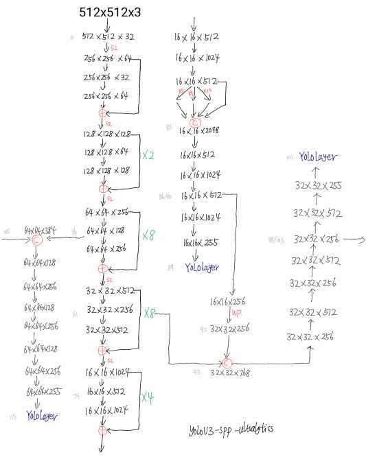
这里贴一张 ‘cfg/yolov3-spp.cfg‘ 网络结构示意图:
具体实现参考 models.py 这份代码。这里有个有意思的地方是默认会使用 thop 按照固定输入(1, 3, 480, 640)尺度统计参数量和计算量,看来在 pytorch 中 thop 的使用率还是挺高的。
imgsz 这个参数目的是为了 onnx 准备的,因为要固定输入尺寸。
dataset = LoadImages(source, img_size=imgsz)
这里的数据预处理包括 padding_resize 和 BGR2EGB,具体参考 utils/datasets.py。推理前图片还要经过 img /= 255.0 归一化操作,就是不知道为什么作者不把这个操作放到 datasets.py 里了。
除了常规的前向推理外,代码中还定义了一种 Augment images 推理方式,有兴趣的可以去瞅瞅。主要关注的是 YOLOLayer 层的推理,这基本上和 TensorFlow 版本 的差不多 。
YOLOV3 有三个尺度的预测输出,以上面图示 512x512 尺度的输入,coco 数据集训练的模型的第一个尺度(最小 feature map) 输出为例。YOLOLayer 前一层的输出维度为 16 x 16 x 255,16 x 16 对应的是 feature map size,255=3*(4+1+80),其中 3 是由于每个尺度上设计了 3 种 Anchor, 4 分别是中心点xy的偏移、宽高的偏移量,1 代表是否包含目标,80 则是具体类别的置信度。
流程上作者将 YOLOLayer 前一层的输出维度进行变换:
# p.view(bs, 255, 16, 16) -- > (bs, 3, 16, 16, 85)  # (bs, anchors, grid, grid, xywh + classes)
p = p.view(bs, self.na, self.no, self.ny, self.nx).permute(0, 1, 3, 4, 2).contiguous()  # prediction
随后按照论文中的方式对预测结果进行 decode:
io = p.clone()  # inference output
io[..., :2] = torch.sigmoid(io[..., :2]) + self.grid  # xy
io[..., 2:4] = torch.exp(io[..., 2:4]) * self.anchor_wh  # wh yolo method
io[..., :4] *= self.stride
torch.sigmoid_(io[..., 4:]) # 会改变 io
return io.view(bs, -1, self.no), p  # view [1, 3, 16, 16, 85] as [1, 768, 85]
具体实现参考 models.py
训练这块算是这个版本的亮点之处了,相比于官方 Darknet 改进点还是很多的。
# Dataset
dataset = LoadImagesAndLabels(train_path, img_size, batch_size,
                              augment=True,
                              hyp=hyp,  # augmentation hyperparameters
                              rect=opt.rect,  # rectangular training
                              cache_images=opt.cache_images,
                              single_cls=opt.single_cls)

# Dataloader
batch_size = min(batch_size, len(dataset))
nw = min([os.cpu_count(), batch_size if batch_size > 1 else 0, 8])  # number of workers
dataloader = torch.utils.data.DataLoader(dataset,
                                         batch_size=batch_size,
                                         num_workers=nw,
                                         shuffle=not opt.rect,  # Shuffle=True unless rectangular training is used
                                         pin_memory=True,
                                         collate_fn=dataset.collate_fn)
区别于推理环节只需要加载和处理图片,这里加载的是类似于 COO 的数据集。以训练 coco2017.data 为例,训练数据 train_path 保存的是训练集的图片路径,LoadImagesAndLabels 中会对应加载 txt 格式的标注文件。
以 train2017/000000391895.jpg 为例,标注文件格式如下 (cx, cy, w, h)
3 0.6490546875000001 0.7026527777777778 0.17570312500000002 0.59325
0 0.65128125 0.47923611111111114 0.2404375 0.8353611111111112
0 0.765 0.5468611111111111 0.05612500000000001 0.13361111111111112
1 0.7833203125 0.5577777777777778 0.047859375 0.09716666666666667
该图片尺寸(HxW)为 360x640, 训练时如果设置的训练尺度为 512,那么这张图片需要先保持高宽比缩放到 288x512 然后再 padding 到 512x512,当然对应的 label 也要有所调整,最后图片要 BGR2EGB 转换。
数据增广包括:
具体参考 utils/datasets.py。
考虑到存在 crop 形式的数据增广,这里区别于 TensorFlow 版本 并没有在数据层就把 Anchor 匹配给做了,而是在训练中做了。
比较有特点的是,代码中将可训练的参数划分为三组,卷积层权重为一组,bias 为一组,其它的参数为一组
pg0, pg1, pg2 = [], [], []  # optimizer parameter groups
for k, v in dict(model.named_parameters()).items():
    if ‘.bias‘ in k:
        pg2 += [v]  # biases
    elif ‘Conv2d.weight‘ in k:
        pg1 += [v]  # apply weight_decay
    else:
        pg0 += [v]  # all else
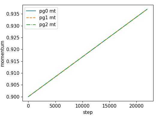
训练中,这三组参数设置不同学习速率
if opt.adam:
    # hyp[‘lr0‘] *= 0.1  # reduce lr (i.e. SGD=5E-3, Adam=5E-4)
    optimizer = optim.Adam(pg0, lr=hyp[‘lr0‘])
    # optimizer = AdaBound(pg0, lr=hyp[‘lr0‘], final_lr=0.1)
else:
    # momentum 一次设置后面都默认是这么多
    optimizer = optim.SGD(pg0, lr=hyp[‘lr0‘], momentum=hyp[‘momentum‘], nesterov=True)
optimizer.add_param_group({‘params‘: pg1, ‘weight_decay‘: hyp[‘weight_decay‘]})  # add pg1 with weight_decay
optimizer.add_param_group({‘params‘: pg2})  # add pg2 (biases)
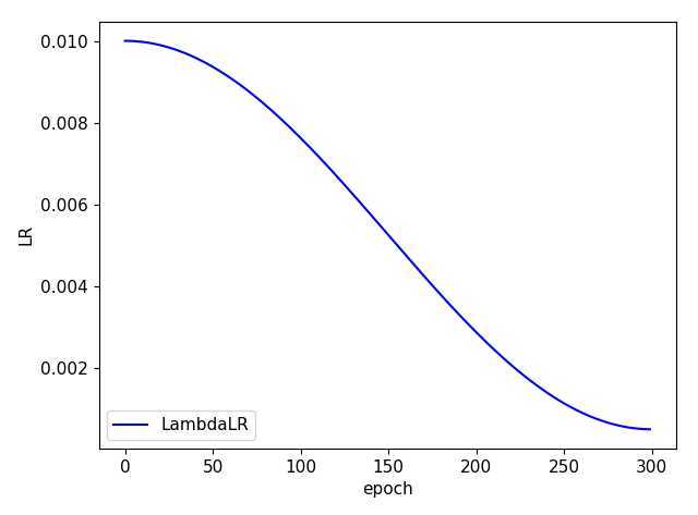
基础学习率采用 cosine
lf = lambda x: (((1 + math.cos(x * math.pi / epochs)) / 2) ** 1.0) * 0.95 + 0.05 # cosine
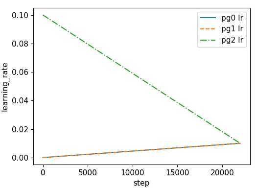
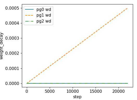
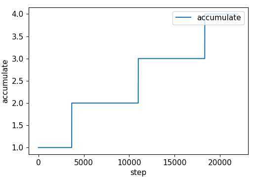
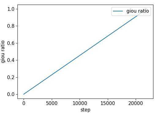
同时,代码中也设计了 warmup 训练方式:
nb = len(dataloader)  # number of batches
n_burn = max(3 * nb, 500)
# Burn-in
if ni <= n_burn:
    xi = [0, n_burn]  # x interp
    model.gr = np.interp(ni, xi, [0.0, 1.0])  # giou loss ratio (obj_loss = 1.0 or giou)
    accumulate = max(1, np.interp(ni, xi, [1, 64 / batch_size]).round())
    for j, x in enumerate(optimizer.param_groups): # pg0 pg1 pg2
        # bias lr falls from 0.1 to lr0, all other lrs rise from 0.0 to lr0
        x[‘lr‘] = np.interp(ni, xi, [0.1 if j == 2 else 0.0, x[‘initial_lr‘] * lf(epoch)])
        x[‘weight_decay‘] = np.interp(ni, xi, [0.0, hyp[‘weight_decay‘] if j == 1 else 0.0])
        if ‘momentum‘ in x:
            x[‘momentum‘] = np.interp(ni, xi, [0.9, hyp[‘momentum‘]])
| learning rate | weight decay |
 |
 |
| momentum | accumulate |
 |
 |
model.gr |
|
 |
值得注意的是:Optimize 是每隔 accumulate 个 batch 才更新模型的,也就是说不考虑 warmup 的情况下,训练的实际 batch_size = 64。
accumulate = max(round(64 / batch_size), 1)
同其它版本一样,这份代码也支持多尺度训练,且是每 effective bs = batch_size * accumulate 更新一次训练尺度
训练还采用了 Model Exponential Moving Average 机制
除了一些预定义的超参数外,还要关注下 model.gr 和 model.class_weights,同预定义的 cls, cls_pw, obj, obj_pw 一样这些都是计算 loss 所准备的一些权重项
model.gr = 1.0  # giou loss ratio (obj_loss = 1.0 or giou)
model.class_weights = labels_to_class_weights(dataset.labels, nc).to(device)  # attach class weights
loss, loss_items = compute_loss(pred, targets, model)
这部分定义在 utils/utils.py 文件中。
首先将 Anchor 和 GT 尝试进行匹配,匹配方式是中心点方式匹配,这里存在一个隐含的风险是有可能存在 GT 没有任何匹配 Anchor,其他版本中是会为该 GT 寻找一个最大匹配项,这里没有,默认舍弃了。
匹配函数:

def build_targets(p, targets, model):
    # Build targets for compute_loss(), input targets(image,class,x,y,w,h)
    nt = targets.shape[0]
    tcls, tbox, indices, anch = [], [], [], []
    gain = torch.ones(6, device=targets.device)  # normalized to gridspace gain
    off = torch.tensor([[1, 0], [0, 1], [-1, 0], [0, -1]], device=targets.device).float()  # overlap offsets

    style = None
    multi_gpu = type(model) in (nn.parallel.DataParallel, nn.parallel.DistributedDataParallel)
    for i, j in enumerate(model.yolo_layers): # 每个尺度输出
        anchors = model.module.module_list[j].anchor_vec if multi_gpu else model.module_list[j].anchor_vec
        gain[2:] = torch.tensor(p[i].shape)[[3, 2, 3, 2]]  # xyxy gain
        na = anchors.shape[0]  # number of anchors
        at = torch.arange(na).view(na, 1).repeat(1, nt)  # anchor tensor, same as .repeat_interleave(nt)

        # Match targets to anchors
        a, t, offsets = [], targets * gain, 0
        if nt:
            # r = t[None, :, 4:6] / anchors[:, None]  # wh ratio
            # j = torch.max(r, 1. / r).max(2)[0] < model.hyp[‘anchor_t‘]  # compare
            j = wh_iou(anchors, t[:, 4:6]) > model.hyp[‘iou_t‘]  # iou(3,n) = wh_iou(anchors(3,2), gwh(n,2))
            a, t = at[j], t.repeat(na, 1, 1)[j]  # filter

            # overlaps
            gxy = t[:, 2:4]  # grid xy
            z = torch.zeros_like(gxy)
            if style == ‘rect2‘:
                g = 0.2  # offset
                j, k = ((gxy % 1. < g) & (gxy > 1.)).T
                a, t = torch.cat((a, a[j], a[k]), 0), torch.cat((t, t[j], t[k]), 0)
                offsets = torch.cat((z, z[j] + off[0], z[k] + off[1]), 0) * g

            elif style == ‘rect4‘:
                g = 0.5  # offset
                j, k = ((gxy % 1. < g) & (gxy > 1.)).T
                l, m = ((gxy % 1. > (1 - g)) & (gxy < (gain[[2, 3]] - 1.))).T
                a, t = torch.cat((a, a[j], a[k], a[l], a[m]), 0), torch.cat((t, t[j], t[k], t[l], t[m]), 0)
                offsets = torch.cat((z, z[j] + off[0], z[k] + off[1], z[l] + off[2], z[m] + off[3]), 0) * g

        # Define
        b, c = t[:, :2].long().T  # image, class
        gxy = t[:, 2:4]  # grid xy
        gwh = t[:, 4:6]  # grid wh
        gij = (gxy - offsets).long()
        gi, gj = gij.T  # grid xy indices

        # Append
        indices.append((b, a, gj, gi))  # image, anchor, grid indices
        tbox.append(torch.cat((gxy - gij, gwh), 1))  # box
        anch.append(anchors[a])  # anchors
        tcls.append(c)  # class
        if c.shape[0]:  # if any targets
            assert c.max() < model.nc, ‘Model accepts %g classes labeled from 0-%g, however you labelled a class %g. ‘                                        ‘See https://github.com/ultralytics/yolov3/wiki/Train-Custom-Data‘ % (
                                           model.nc, model.nc - 1, c.max())

    return tcls, tbox, indices, anch
匹配函数返回四个变量 tcls, tbox, indices, anchors,还是以上面的示例 GT 同第一个尺度的 Anchor 匹配为例:
Anchor 预定义如下,标记部分是第一个尺度(最小 featuremap 用来检测大目标):
anchors = 10,13, 16,30, 33,23, 30,61, 62,45, 59,119, 116,90, 156,198, 373,326
1. 将这个尺度的 Anchor 映射到该 featuremap 尺度得到 anchors
2. 将 GT 映射到该 featuremap 尺度得到 t
3. 中心点方式匹配 ($Anchor_{num} x GT_{num}$)

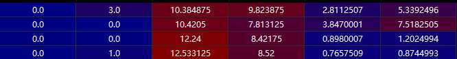
这样的话匹配的 Anchor 索引 a=[0, 0,1,1, 2] 和 GT 为 下图 t,b 和 c 则分别代表匹配的 GT 在一个 batch 中的 index 和 类别 id:
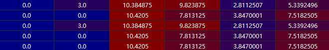
b c
gij 计统计的是匹配的 GT 的中心点坐标,gi, gj 分别是 center_x 和 center_y
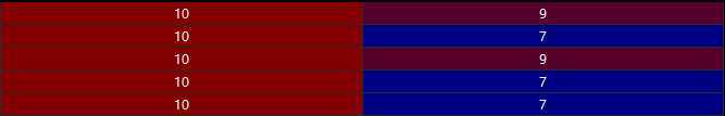
gi gj
最后输出的四个变量如下
tcls.append(c)  # class
tbox.append(torch.cat((gxy - gij, gwh), 1))  # box
indices.append((b, a, gj, gi))  # image, anchor, grid indices
anch.append(anchors[a])  # anchors
To be continue...
原文:https://www.cnblogs.com/xuanyuyt/p/13037101.html
