线性模型:
数据集:\(D = \{(\boldsymbol{x}_1, y_1), (\boldsymbol{x}_2, y_2), ... , (\boldsymbol{x}_m, y_m)\}\),\(\boldsymbol{x}_i = (x_{i1}; x_{i2};...; x_{id})\)
损失函数 (Loss function) 采用平方损失:
目标是找到一组解 \((\boldsymbol{w}^{\star}, b^{\star})\) 使得损失函数的值最小,即:
求解方法:
损失函数的代码实现:
import numpy as np
import matplotlib.pyplot as plt
import pandas as pd
import math
import random
# 误差函数
def loss_function(w, b, x, y):
  x = np.array(x)
  y = np.array(y).reshape(len(y), 1)
  w = np.array(w)
  b = np.array(b)

  x = np.matrix(x)
  y = np.matrix(y)
  w = np.matrix(w)
  b = np.matrix(b)

  err = [[0.0]]
  m = len(x)
  for i in range(m):
    err = err + (y[i] - w.T * x[i] - b) ** 2
    # err = err + abs(y[i,:] - w.T * x[i,:] - b)
  return err.tolist()[0][0]

# 误差函数重载,这里的w包含了w和b
def loss_function(w, x, y):
  x = np.array(x)
  y = np.array(y).reshape(len(y), 1)
  w = np.array(w)

  x=np.concatenate((x, np.ones((len(x), 1))), axis=1)

  x = np.matrix(x)
  y = np.matrix(y)
  w = np.matrix(w)
  # print(w)

  err = 0.0
  m = len(x)
  # print(‘-------‘)
  # print(m)
  for i in range(m):
    pp= x[i] * w
    p=(y[i] - pp.T )
    err = err + p * p.T
    # err = err + (y[i] - x[i] * w.T ) ** 2
  # return math.sqrt(err.tolist()[0][0])/10
  return err.tolist()[0][0]
#测试

x = [ [1.], [2.]]
y = [ 1., 2.]

print(loss_function([1], 0, x, y))
运行结果为:
0.0
把 \(\boldsymbol{w}\) 和 \(b\) 吸收入向量形式 \(\hat{\boldsymbol{w}} = (\boldsymbol{w}; b)\)
把数据集 \(D\) 的输入表示为一个 \(m \times (d + 1)\) 大小的矩阵 \(\boldsymbol{X}\)
把输出也表示成向量形式 \(\boldsymbol{y} = (y_1; y_2; ...; y_n)\)
式(2) 可表示为
式(3) 可表示为
对式(4)求导可得
当 \(\boldsymbol{X}^T\boldsymbol{X}\) 为满秩矩阵时(不是满秩矩阵时无法求解),令式(5)等于0可得解为
Python代码实现:
import numpy as np
from numpy import *
# 求解
def get_w(x, y):
  w = (x.T * x).I * x.T * y
  return w.tolist()

# 最小二乘法
def least_squares(x, y):
  x = np.array(x)

  x = np.concatenate((x, np.ones((len(x), 1))), axis=1)

  x = np.matrix(x)
  # print(x)


  y = np.array(y).reshape(len(y), 1)
  y = np.matrix(y)
  # print(y)

  return get_w(x, y)
# 测试
# x = [[1], [2], [3]]
# y = [1, 2, 3]

x = [ [338.], [333.], [328.], [207.], [226.], [25.], [179.], [60.], [208.], [606.]]
y = [ 640., 633., 619., 393., 428., 27., 193., 66., 226., 1591.]

w = least_squares(x, y)
w0 = w[0:len(w) - 1][0]

print(math.sqrt(loss_function(w0, w[-1][0], x, y)) / len(x))
运行结果为:
31.927531989787543
# 画图

x_list = []
y_list = y

for i in x:
  x_list.append(i[0])

#创建图
ax = plt.gca()
#设置x轴、y轴名称
ax.set_xlabel(‘x‘)
ax.set_ylabel(‘y‘)

#画散点图,以x_list中的值为横坐标,以y_list中的值为纵坐标
#参数c指定点的颜色,s指定点的大小,alpha指定点的透明度
ax.scatter(x_list, y_list, c=‘r‘, s=20, alpha=0.5)

print(str(w[0][0]) + ‘ ‘ + str(w[1][0]))

p1 = [0, 600]
p2 = [0 * w[0][0] + w[1][0], 600 * w[0][0] + w[1][0]]

ax1 = plt.gca()
#设置x轴、y轴名称
ax1.set_xlabel(‘x‘)
ax1.set_ylabel(‘y‘)

#参数c指定连线的颜色,linewidth指定连线宽度,alpha指定连线的透明度
ax1.plot(p1, p2, color=‘b‘, linewidth=1, alpha=0.6)

plt.show()
模型的解为:
2.669454966762257 -188.43319665732653
采用statsmodels库求线性回归作为对比:
# 采用statsmodels库求线性回归
import statsmodels.api as sm
import matplotlib.pyplot as plt

x = [ [338.], [333.], [328.], [207.], [226.], [25.], [179.], [60.], [208.], [606.]]
y = [ 640., 633., 619., 393., 428., 27., 193., 66., 226., 1591.]
x = sm.add_constant(x) # 若模型中有截距,必须有这一步
model = sm.OLS(y, x).fit() # 构建最小二乘模型并拟合
print(model.summary()) # 输出回归结果
                            OLS Regression Results
==============================================================================
Dep. Variable:                      y   R-squared:                       0.944
Model:                            OLS   Adj. R-squared:                  0.938
Method:                 Least Squares   F-statistic:                     136.1
Date:                Wed, 10 Jun 2020   Prob (F-statistic):           2.66e-06
Time:                        07:28:51   Log-Likelihood:                -60.337
No. Observations:                  10   AIC:                             124.7
Df Residuals:                       8   BIC:                             125.3
Df Model:                           1
Covariance Type:            nonrobust
==============================================================================
                 coef    std err          t      P>|t|      [0.025      0.975]
------------------------------------------------------------------------------
const       -188.4332     67.619     -2.787      0.024    -344.363     -32.503
x1             2.6695      0.229     11.667      0.000       2.142       3.197
==============================================================================
Omnibus:                        1.562   Durbin-Watson:                   2.661
Prob(Omnibus):                  0.458   Jarque-Bera (JB):                0.877
Skew:                           0.356   Prob(JB):                        0.645
Kurtosis:                       1.737   Cond. No.                         560.
==============================================================================

Warnings:
[1] Standard Errors assume that the covariance matrix of the errors is correctly specified.


/usr/local/lib/python3.6/dist-packages/scipy/stats/stats.py:1535: UserWarning: kurtosistest only valid for n>=20 ... continuing anyway, n=10
  "anyway, n=%i" % int(n))
可以看到结果基本一致。
式(4)的梯度为
根据梯度下降法,不断更新 \(\hat{\boldsymbol{w}}\) 去寻找 \(\hat{\boldsymbol{w}}^*\)。参数的更新以目标的负梯度为方向,\(t\) 表示第 \(t\) 次更新参数,\(\eta\) 表示学习率。
Python代码实现:
import numpy as np
import matplotlib.pyplot as plt
import pandas as pd
# 梯度
def gradient(w, x, y):
  x = np.array(x)
  y = np.array(y).reshape(len(y), 1)
  x = np.concatenate((x, np.ones((len(x), 1))), axis=1)
  w = np.array(w)

  x = np.matrix(x)
  y = np.matrix(y)
  w = np.matrix(w)

  # print(w)
  return 2 * x.T * (x * w - y)

# 梯度下降
def gradient_descent(x, y):
  lr = 0.0000001  # learning rate
  iteration = 1000000  # 迭代次数
  w = np.ones((1, len(x[0]) + 1)).T
  w[len(x[0])][0] = y[0] - x[0][0]
  # w=data.iloc[1:2,1:-1].values
  # w=np.concatenate((w, np.ones((len(w), 1))), axis=1).T
  # print(x)
  # print(w)

  for i in range(iteration):
    w = w - lr * gradient(w, x, y)

  return w
测试结果:
# 测试
# data=pd.read_csv(‘final_data.csv‘,encoding=‘gb18030‘)
# x = data.iloc[:,1:-1].values
# y = data.iloc[:,0].values

# print(x)
# print(y)

x = [ [338.], [333.], [328.], [207.], [226.], [25.], [179.], [60.], [208.], [606.]]
y = [ 640., 633., 619., 393., 428., 27., 193., 66., 226., 1591.]

w = gradient_descent(x, y)
w = w.tolist()

print(w)

w0 = w[0:len(w) - 1][0]

# print(math.sqrt(loss_function(w0, w[-1][0], x, y)) / len(x))
print(math.sqrt(loss_function(w, x, y)) / len(x))  # 均方误差
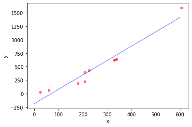
模型的解及误差为:
[[2.664103150270952], [-186.57092397847248]]
31.929045483933738
# 画图

x_list = []
y_list = y

for i in x:
  x_list.append(i[0])

#创建图
ax = plt.gca()
#设置x轴、y轴名称
ax.set_xlabel(‘x‘)
ax.set_ylabel(‘y‘)

#画散点图,以x_list中的值为横坐标,以y_list中的值为纵坐标
#参数c指定点的颜色,s指定点的大小,alpha指定点的透明度
ax.scatter(x_list, y_list, c=‘r‘, s=20, alpha=0.5)

print(str(w[0][0]) + ‘ ‘ + str(w[1][0]))

p1 = [0, 600]
p2 = [0 * w[0][0] + w[1][0], 600 * w[0][0] + w[1][0]]

ax1 = plt.gca()
#设置x轴、y轴名称
ax1.set_xlabel(‘x‘)
ax1.set_ylabel(‘y‘)

#参数c指定连线的颜色,linewidth指定连线宽度,alpha指定连线的透明度
ax1.plot(p1, p2, color=‘b‘, linewidth=1, alpha=0.6)

plt.show()
2.664103150270952 -186.57092397847248

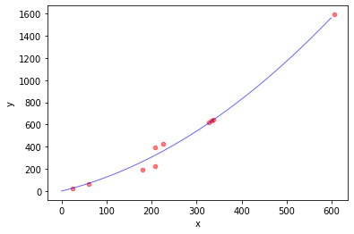
线性回归也可以求解非线性模型。如引入二次项:
可以把 \(x_i^2\) 看成另一个特征,本质还是线性回归
# 梯度下降
def gradient_descent(x, y):
  lr = 1e-12  # learning rate
  iteration = 1000000  # 迭代次数
  w = np.ones((1, len(x[0]) + 1)).T

  for i in range(iteration):
    w = w - lr * gradient(w, x, y)

  return w

x = [ [338.], [333.], [328.], [207.], [226.], [25.], [179.], [60.], [208.], [606.]]
y = [ 640., 633., 619., 393., 428., 27., 193., 66., 226., 1591.]

m = len(x)
for i in range(m - 1, -1, -1):
  x[i].insert(0, x[i][0] ** 2)

print(x)
print(y)

w = gradient_descent(x, y)
w = w.tolist()

print(w)

w0 = w[0:len(w) - 1][0]

# print(math.sqrt(loss_function(w0, w[-1][0], x, y)) / len(x))
print(math.sqrt(loss_function(w, x, y)) / len(x))  # 均方误差
[[114244.0, 338.0], [110889.0, 333.0], [107584.0, 328.0], [42849.0, 207.0], [51076.0, 226.0], [625.0, 25.0], [32041.0, 179.0], [3600.0, 60.0], [43264.0, 208.0], [367236.0, 606.0]]
[640.0, 633.0, 619.0, 393.0, 428.0, 27.0, 193.0, 66.0, 226.0, 1591.0]
[[0.002695722750670167], [0.9906491919888195], [0.9999201489658276]]
15.529527888679146
可以看到误差小了一半。
# 画图

x_list = []
y_list = y

for i in x:
  x_list.append(i[1])

#创建图
ax = plt.gca()
#设置x轴、y轴名称
ax.set_xlabel(‘x‘)
ax.set_ylabel(‘y‘)

#画散点图,以x_list中的值为横坐标,以y_list中的值为纵坐标
#参数c指定点的颜色,s指定点的大小,alpha指定点的透明度
ax.scatter(x_list, y_list, c=‘r‘, s=20, alpha=0.5)


# p1 = [0, 600]
# p2 = [0 * w[0][0] + w[1][0], 600 * w[0][0] + w[1][0]]
p1 = []
p2 = []

print(w[0][0])
print(w[1][0])
print(w[2][0])

for i in range(600):
  p1.append(i)
  p2.append(i * i * w[0][0] + i * w[1][0] + w[2][0])

# print(p1)
# print(p2)


ax1 = plt.gca()
#设置x轴、y轴名称
ax1.set_xlabel(‘x‘)
ax1.set_ylabel(‘y‘)

#参数c指定连线的颜色,linewidth指定连线宽度,alpha指定连线的透明度
ax1.plot(p1, p2, color=‘b‘, linewidth=1, alpha=0.6)

plt.show()
模型的解为:
0.002695722750670167
0.9906491919888195
0.9999201489658276
模拟退火算法基于物理退火的原理,将固体加热至高温然后冷却,温度越高降温的概率越大 (降温更快),温度越低降温的概率越小 (降温越慢)。模拟退火算法进行多次降温,直到找到一个可行解。
简单来说,如果新的状态比当前状态更优就接受该状态,否则以一定概率接受新状态。概率为:\(P(\Delta E) = e^{\frac{-\Delta E}{T}}\),其中 \(T\) 为当前温度,\(\Delta E\) 新状态与当前状态的能量差。
模拟退火主要有三个参数:初始温度 \(T_0\),降温系数 \(d\),终止温度 \(T_k\)。
让当前温度 \(T = T_0\),温度下降,尝试转移,如果转移 \(T = d * T\)。当 \(T < T_k\) 时结束模拟退火算法。
# 模拟退火
def simulateAnneal(x, y):
  Tk = 1e-8  # 终止温度
  T0 = 100  # 初始温度
  d = 0.5  # 降温系数
  w = [[1] for i in range(len(x[0]) + 1)]
  # now = loss_function(w, x, y)
  # nxt = now
  # min_value = now  # 损失函数最小值

  min_value = loss_function(w, x, y)  # 损失函数最小值
  T = T0  # 当前温度
  cnt = 0  # 迭代次数
  while T > Tk:
    cnt += 1
    next = []
    mn = 1e20  # 临时的最小值
    for i in range(50):
      nw = []
      for i in w:
        nw.append(i.copy())

      for i in range(len(w)):
        nw[i][0] = w[i][0] + math.cos(myrand() * 2 * math.pi) * T

      nE = loss_function(nw, x, y)  # 新状态

      if mn > nE:  # 更新最小值
        mn = nE
        next = []
        for i in nw:
          next.append(i.copy())
    dE = mn - min_value  # 能量差
    if dE / T > 0:
      continue
    if dE < 0 or math.exp(dE / T) < myrand():
      min_value = mn
      w = []
      for i in next:
        w.append(i.copy())
    T = T * d  # 降温
  print(cnt)
  return w

def myrand():
  return random.randint(0, 10000) / 10000;
# 测试
x = [ [338.], [333.], [328.], [207.], [226.], [25.], [179.], [60.], [208.], [606.]]
y = [ 640., 633., 619., 393., 428., 27., 193., 66., 226., 1591.]

w = simulateAnneal(x, y)
# w = w.tolist()

print(w)

print(math.sqrt(loss_function(w, x, y)) / len(x))
40
[[2.5460349824125927], [-145.48637019150746]]
32.72257883908066
模拟退火求得的解随机性比较强,可能效果很好也可能很差,因为模拟退火能跳出局部最优解,也可能跳出全局最优解。
随机梯度下降法在计算梯度时加入随机因素,这样即便陷入局部最小点,计算出的梯度仍可能不为零,就有机会跳出局部极小继续搜索。
# 梯度
def gradient(w, x, y):
  x = np.array(x)
  y = np.array(y).reshape(len(y), 1)
  x = np.concatenate((x, np.ones((len(x), 1))), axis=1)
  w = np.array(w)

  x = np.matrix(x)
  y = np.matrix(y)
  w = np.matrix(w)
  # print(w)
  return 2 * x.T * (x * w - y)

# 随机梯度下降
def random_gradient_descent(x, y):
  lr = 0.0000001  # learning rate
  iteration = 1000000
  w = np.ones((1, len(x[0]) + 1)).T
  w[len(x[0])][0] = y[0] - x[0][0]

  for i in range(iteration):
    id = random.randint(0, len(x) - 1)  # 随机选择一组数据
    w = w - lr * gradient(w, [x[id]], [y[id]])

  return w
# 测试
x = [ [338.], [333.], [328.], [207.], [226.], [25.], [179.], [60.], [208.], [606.]]
y = [ 640., 633., 619., 393., 428., 27., 193., 66., 226., 1591.]

w = random_gradient_descent(x, y)
w = w.tolist()

print(w)

w0 = w[0:len(w) - 1][0]

# print(math.sqrt(loss_function(w0, w[-1][0], x, y)) / len(x))
print(math.sqrt(loss_function(w, x, y)) / len(x))
[[1.4345358411567755], [275.41894946969995]]
84.25783548408097
原文:https://www.cnblogs.com/wulitaotao/p/13173890.html