自然语言推理:使用注意力机制
Natural Language Inference: Using Attention
自然语言推理任务和SNLI数据集。鉴于许多模型都是基于复杂和深层架构的,Parikh等人提出用注意机制解决自然语言推理问题,并称之为“可分解注意力模型”【Parikh等人,2016年】。这就产生了一个没有递归层或卷积层的模型,在SNLI数据集上用更少的参数获得了最好的结果。在本节中,将描述并实现这种基于注意的自然语言推理方法(使用MLPs),如图1所示。
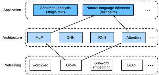
Fig. 1. This section feeds pretrained GloVe to an architecture based on attention and MLPs for natural language inference.
1. The Model
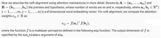
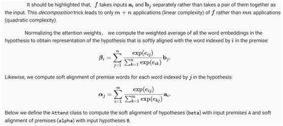
比起在前提和假设中保持单词的顺序更简单,可以将一个文本序列中的单词与另一个文本序列中的每个单词对齐,反之亦然,然后比较和聚合这些信息来预测前提和假设之间的逻辑关系。与机器翻译中源句子和目标句子之间的单词对齐类似,前提和假设之间的单词对齐也可以通过注意机制来完成。
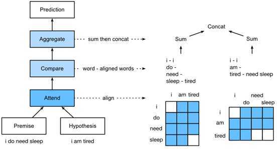
Fig. 2. Natural language inference using attention mechanisms.
图2描述了使用注意机制的自然语言推理方法。在高层次上,包括三个共同训练的步骤:参与、比较和汇总。将在下面一步一步地加以说明。
from d2l import mxnet as d2l
import mxnet as mx
from mxnet import autograd, gluon, init, np, npx
from mxnet.gluon import nn
npx.set_np()
1.1. Attending
第一步是将一个文本序列中的单词与另一个序列中的每个单词对齐。假设前提是“确实需要睡眠”,假设是“累了”。由于语义上的相似性,可以将假设中的“”与前提中的“”对齐,将假设中的“累”与前提中的“睡眠”对齐。同样,也可以将前提中的“”与假设中的“”对齐,并将前提中的“需要”和“睡眠”与假设中的“累”对齐。注意,这种对齐使用加权平均是软的,在理想情况下,较大的权重与要对齐的单词相关联。为了便于演示,图2以硬的方式显示了这种对齐方式。
def mlp(num_hiddens, flatten):
net = nn.Sequential()
net.add(nn.Dropout(0.2))
net.add(nn.Dense(num_hiddens, activation=‘relu‘, flatten=flatten))
net.add(nn.Dropout(0.2))
net.add(nn.Dense(num_hiddens, activation=‘relu‘, flatten=flatten))
return net
class Attend(nn.Block):
def __init__(self, num_hiddens, **kwargs):
super(Attend, self).__init__(**kwargs)
self.f = mlp(num_hiddens=num_hiddens, flatten=False)
def forward(self, A, B):
# Shape of A/B: (batch_size, #words in sequence A/B, embed_size)
# Shape of f_A/f_B: (batch_size, #words in sequence A/B, num_hiddens)
f_A = self.f(A)
f_B = self.f(B)
# Shape of e: (batch_size, #words in sequence A, #words in sequence B)
e = npx.batch_dot(f_A, f_B, transpose_b=True)
# Shape of beta: (batch_size, #words in sequence A, embed_size), where
# sequence B is softly aligned with each word (axis 1 of beta) in
# sequence A
beta = npx.batch_dot(npx.softmax(e), B)
# Shape of alpha: (batch_size, #words in sequence B, embed_size),
# where sequence A is softly aligned with each word (axis 1 of alpha)
# in sequence B
alpha = npx.batch_dot(npx.softmax(e.transpose(0, 2, 1)), A)
return beta, alpha
1.2. Comparing
在下一步中,将一个序列中的一个单词与另一个与该单词轻轻对齐的序列进行比较。请注意,在软对齐中,来自一个序列的所有单词,尽管可能具有不同的注意权重,但将与另一个序列中的一个单词进行比较。为了便于演示,图15.5.2将单词与对齐的单词进行硬配对。例如,假设主治步骤确定前提中的“需要”和“睡眠”都与假设中的“累”一致,则将对“累-需要睡眠”进行比较。
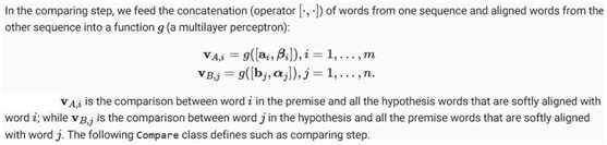
在比较步骤中,提供连接(运算符 [⋅,⋅])将一个序列中的单词和另一个序列中的对齐单词组合成一个函数g(多层感知器):
class Compare(nn.Block):
def __init__(self, num_hiddens, **kwargs):
super(Compare, self).__init__(**kwargs)
self.g = mlp(num_hiddens=num_hiddens, flatten=False)
def forward(self, A, B, beta, alpha):
V_A = self.g(np.concatenate([A, beta], axis=2))
V_B = self.g(np.concatenate([B, alpha], axis=2))
return V_A, V_B
1.3. Aggregating
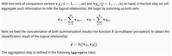
class Aggregate(nn.Block):
def __init__(self, num_hiddens, num_outputs, **kwargs):
super(Aggregate, self).__init__(**kwargs)
self.h = mlp(num_hiddens=num_hiddens, flatten=True)
self.h.add(nn.Dense(num_outputs))
def forward(self, V_A, V_B):
# Sum up both sets of comparison vectors
V_A = V_A.sum(axis=1)
V_B = V_B.sum(axis=1)
# Feed the concatenation of both summarization results into an MLP
Y_hat = self.h(np.concatenate([V_A, V_B], axis=1))
return Y_hat
1.4. Putting All Things Together
通过将参与、比较和聚合步骤放在一起,定义了可分解的注意力模型来联合训练这三个步骤。
class DecomposableAttention(nn.Block):
def __init__(self, vocab, embed_size, num_hiddens, **kwargs):
super(DecomposableAttention, self).__init__(**kwargs)
self.embedding = nn.Embedding(len(vocab), embed_size)
self.attend = Attend(num_hiddens)
self.compare = Compare(num_hiddens)
# There are 3 possible outputs: entailment, contradiction, and neutral
self.aggregate = Aggregate(num_hiddens, 3)
def forward(self, X):
premises, hypotheses = X
A = self.embedding(premises)
B = self.embedding(hypotheses)
beta, alpha = self.attend(A, B)
V_A, V_B = self.compare(A, B, beta, alpha)
Y_hat = self.aggregate(V_A, V_B)
return Y_hat
2. Training and Evaluating the Model
现在将在SNLI数据集上训练和评估已定义的可分解注意力模型。从读取数据集开始。
2.1. Reading the dataset
下载并读取SNLI数据集。批大小和序列长度分别设置为256和50。
batch_size, num_steps = 256, 50
train_iter, test_iter, vocab = d2l.load_data_snli(batch_size, num_steps)
read 549367 examples
read 9824 examples
2.2. Creating the Model
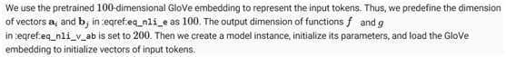
embed_size, num_hiddens, ctx = 100, 200, d2l.try_all_gpus()
net = DecomposableAttention(vocab, embed_size, num_hiddens)
net.initialize(init.Xavier(), ctx=ctx)
glove_embedding = d2l.TokenEmbedding(‘glove.6b.100d‘)
embeds = glove_embedding[vocab.idx_to_token]
net.embedding.weight.set_data(embeds)
2.3. Training and Evaluating the Model
与split_batch函数不同,该函数采用单个输入,如文本序列(或图像),定义了一个split_batch_multi_inputs函数,以获取多个输入,如小批量中的前提和假设。
#@save
def split_batch_multi_inputs(X, y, ctx_list):
"""Split multi-input X and y into multiple devices specified by ctx"""
X = list(zip(*[gluon.utils.split_and_load(
feature, ctx_list, even_split=False) for feature in X]))
return (X, gluon.utils.split_and_load(y, ctx_list, even_split=False))
现在可以在SNLI数据集上训练和评估模型。
lr, num_epochs = 0.001, 4
trainer = gluon.Trainer(net.collect_params(), ‘adam‘, {‘learning_rate‘: lr})
loss = gluon.loss.SoftmaxCrossEntropyLoss()
d2l.train_ch13(net, train_iter, test_iter, loss, trainer, num_epochs, ctx,
split_batch_multi_inputs)
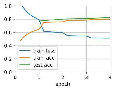
loss 0.511, train acc 0.798, test acc 0.823
9402.9 examples/sec on [gpu(0), gpu(1)]
2.4. Using the Model
最后,定义预测函数,输出一对前提与假设之间的逻辑关系。
#@save
def predict_snli(net, vocab, premise, hypothesis):
premise = np.array(vocab[premise], ctx=d2l.try_gpu())
hypothesis = np.array(vocab[hypothesis], ctx=d2l.try_gpu())
label = np.argmax(net([premise.reshape((1, -1)),
hypothesis.reshape((1, -1))]), axis=1)
return ‘entailment‘ if label == 0 else ‘contradiction‘ if label == 1 \
else ‘neutral‘
利用训练后的模型,可以得到一对例句的自然语言推理结果。
predict_snli(net, vocab, [‘he‘, ‘is‘, ‘good‘, ‘.‘], [‘he‘, ‘is‘, ‘bad‘, ‘.‘])
‘contradiction‘
3. Summary
原文:https://www.cnblogs.com/wujianming-110117/p/13228257.html