Grab算法部分:
import cv2 as cv
import numpy as np


# 鼠标反馈 得到前景矩形起始点,终止点,宽高
def on_mouse(event, x, y, flag, param):
    global rect
    global leftButtonDown
    global leftButtonUp

    if event == cv.EVENT_LBUTTONDOWN:
        rect[0] = x
        rect[2] = x
        rect[1] = y
        rect[3] = y
        leftButtonDown = True
        leftButtonUp = False

    if event == cv.EVENT_MOUSEMOVE:
        if leftButtonDown and not leftButtonUp:
            rect[2] = x
            rect[3] = y

    if event == cv.EVENT_LBUTTONUP:
        if leftButtonDown and not leftButtonUp:
            x_min = min(rect[0], rect[2])
            y_min = min(rect[1], rect[3])
            x_max = max(rect[0], rect[2])
            y_max = max(rect[1], rect[3])

            rect[0] = x_min
            rect[1] = y_min
            rect[2] = x_max
            rect[3] = y_max
            leftButtonUp = True
            leftButtonDown = False


img = cv.imread(‘screenshot.png.jpg‘)
mask = np.zeros(img.shape[:2], np.uint8)

bgdModel = np.zeros((1, 65), np.float64)
fgdModel = np.zeros((1, 65), np.float64)

rect = [0, 0, 0, 0]

leftButtonUp = True
leftButtonDown = False

cv.namedWindow("img")
cv.setMouseCallback("img", on_mouse)
cv.imshow("img", img)

# 实时画出前景矩形,左键放开即开始分离前景
while cv.waitKey(2) == -1:
    if leftButtonDown and not leftButtonUp:
        img_copy = img.copy()
        cv.rectangle(img_copy, (rect[0], rect[1]),
                     (rect[0] + rect[2], rect[1] + rect[3]), (0, 255, 0), 2)
        cv.imshow("img", img_copy)

    if not leftButtonDown and leftButtonUp and rect[0] != 0 and rect[1] != 0:
        rect_copy = tuple(rect.copy())
        print(rect_copy)
        rect = [0, 0, 0, 0]
        cv.grabCut(img, mask, rect_copy, bgdModel, fgdModel, 5, cv.GC_INIT_WITH_RECT)
        # 背景设为0,与原图相乘,则背景为黑色
        mask_two = np.where((mask == 2) | (mask == 0), 0, 1).astype(‘uint8‘)
        img_show = img * mask_two[:, :, np.newaxis]
        cv.imshow("grabcut", img_show)

cv.waitKey()
cv.destroyAllWindows()
分水岭算法:
主要对比了一下案例和网络上另一种用法:
import cv2 as cv
import numpy as np
from matplotlib import pyplot as plt

src = cv.imread("coins.png")
img = src.copy()
gray = cv.cvtColor(img, cv.COLOR_BGR2GRAY)
ret, thresh = cv.threshold(gray, 127, 255, cv.THRESH_BINARY_INV + cv.THRESH_OTSU)
# 开运算
kernel = np.ones((3, 3), np.uint8)
opening = cv.morphologyEx(thresh, cv.MORPH_OPEN, kernel, iterations=2)
# 第二次膨胀
sure_bg = cv.dilate(opening, kernel, iterations=3)
# 距离变换
dist_transform = cv.distanceTransform(opening, cv.DIST_L2, 5)
_, sure_fg = cv.threshold(dist_transform, 0.7 * dist_transform.max(), 255, 0)
sure_fg = np.uint8(sure_fg)
# 边界未知区域
unknown = cv.subtract(sure_bg, sure_fg)
# 标记(会把背景标为0,所以整体加1)
_, markers = cv.connectedComponents(sure_fg)
markers = markers + 1
# 未知区域为0
markers[unknown == 255] = 0
plt.subplot(243), plt.imshow(markers)
# 分水岭
markers = cv.watershed(img, markers)
watershed = cv.convertScaleAbs(markers)
plt.subplot(244), plt.imshow(watershed)
plt.subplot(241), plt.imshow(img)
# 生成随机颜色
colorTab = np.zeros((np.max(markers) + 1, 3))
# 生成0~255之间的随机数
for i in range(len(colorTab)):
    aa = np.random.uniform(0, 255)
    bb = np.random.uniform(0, 255)
    cc = np.random.uniform(0, 255)
    colorTab[i] = np.array([aa, bb, cc], np.uint8)

bgrImage = np.zeros(img.shape, np.uint8)

# 遍历marks每一个元素值,对每一个区域进行颜色填充
for i in range(markers.shape[0]):
    for j in range(markers.shape[1]):
        # index值一样的像素表示在一个区域
        index = markers[i][j]
        # 判断是不是区域与区域之间的分界,如果是边界(-1),则使用白色显示
        if index == -1:
            img[i][j] = np.array([255, 255, 255])
        else:
            img[i][j] = colorTab[index]
plt.subplot(242), plt.imshow(img)


#################################
# canny边缘检测 函数返回一副二值图,其中包含检测出的边缘。
canny = cv.Canny(gray, 80, 150)

# 寻找图像轮廓 返回修改后的图像 图像的轮廓  以及它们的层次
contours, hierarchy = cv.findContours(canny, cv.RETR_TREE, cv.CHAIN_APPROX_SIMPLE)
# 32位有符号整数类型,
marks = np.zeros(img.shape[:2], np.int32)

# 轮廓颜色
compCount = 0
index = 0
# 绘制每一个轮廓
for index in range(len(contours)):
    # 对marks进行标记,对不同区域的轮廓使用不同的亮度绘制,相当于设置注水点,有多少个轮廓,就有多少个轮廓
    # 图像上不同线条的灰度值是不同的,底部略暗,越往上灰度越高
    marks = cv.drawContours(marks, contours, index, (index, index, index), 1, 8, hierarchy)
marks_copy = cv.convertScaleAbs(marks.copy())
plt.subplot(247), plt.imshow(marks_copy)
# 使用分水岭算法
marks = cv.watershed(src, marks)
afterWatershed = cv.convertScaleAbs(marks)
plt.subplot(248), plt.imshow(afterWatershed)

# 生成随机颜色
colorTab = np.zeros((np.max(marks) + 1, 3))
# 生成0~255之间的随机数
for i in range(len(colorTab)):
    aa = np.random.uniform(0, 255)
    bb = np.random.uniform(0, 255)
    cc = np.random.uniform(0, 255)
    colorTab[i] = np.array([aa, bb, cc], np.uint8)

bgrImage = np.zeros(img.shape, np.uint8)

# 遍历marks每一个元素值,对每一个区域进行颜色填充
for i in range(marks.shape[0]):
    for j in range(marks.shape[1]):
        # index值一样的像素表示在一个区域
        index = marks[i][j]
        # 判断是不是区域与区域之间的分界,如果是边界(-1),则使用白色显示
        if index == -1:
            bgrImage[i][j] = np.array([255, 255, 255])
        else:
            bgrImage[i][j] = colorTab[index]


plt.subplot(246), plt.imshow(bgrImage)
plt.show()
cv.waitKey(0)
cv.destroyAllWindows()
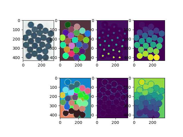
第二列是最终成图,第三列是预处理的markers,第四列是分水岭算法处理后的markers
第一种处理方法的步骤:二值化 => 开运算 => 膨胀 => 距离转换 => 找出位置区域 => 标记区域
第一种处理方法的步骤:canny => 标记轮廓
我们会发现两种思路是完全不同的,第一种重点是圆心的‘水’冲入‘山谷’中,第二种则相反
那么我们会怀疑,第二种既然是边缘‘水’泛滥到圆心,为何还会存在边缘分界呢?
其实是Canny算法将边缘大部分用两条曲线来描述,两股‘水’冲在一起形成分界,但也可看出,Canny效果不好的时候(即只有一条描述边缘),就会在局部形成大面积的泛滥,是极为不理想的效果。(最后一张图下方蓝色区域)
真正运用时,个人认为第一种明显更好,真正做到将每个物体分隔开,而第二种,会发现,如果出现物体粘连,并不能很好地分隔物体(其实没有用好分水岭)。
opencv learning_three ---- 图像分割
原文:https://www.cnblogs.com/zoe1230/p/13538850.html