Multidimensional Signals
In the preceding section we constructed multiamplitude signal waveforms, which allowed
us to transmit multiple bits per signal waveform. Thus, with signal waveforms
having M = 2k(2 power k) amplitude levels, we are able to transmit k = log2 M bits of information
per signal waveform. We also observed that the multiamplitude signals can
be represented geometrically as signal points on the real line. Such signal waveforms are called one-dimensional signals.
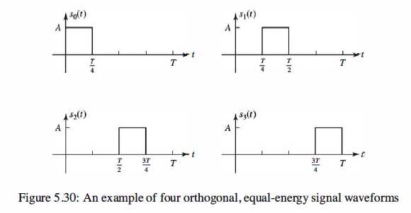
consider the construction of a class of M = 2k(2 power k) signal waveforms
that have a multidimensional representation. That is, the set of signal waveforms
can be represented geometrically as points in N-dimensional space.
Multidimensional Orthogonal Signals
As in our previous discussion, we assume that an information source is providing
a sequence of information bits, which are to be transmitted through a communication
channel. The information bits occur at a uniform rate of R bits per second. The reciprocal
of R is the bit interval, Tb. The modulator takes k bits at a time and maps them
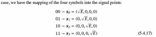
into one of M = 2k(2 power K) signal waveforms. Each block of k bits is called a symbol. The
time interval available to transmit each symbol is T = kTb. Hence, T is the symbol
interval.
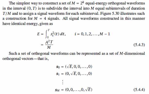
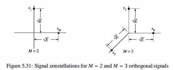
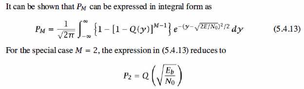
Figure 5 .31 illustrates the signal points (signal constellations) corresponding to M = 2 and M = 3 orthogonal signals.
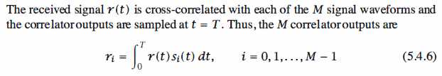
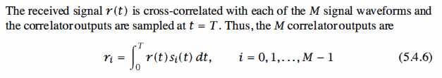
Let us assume that these orthogonal signal waveforms are used to transmit information
through an AWGN channel. Consequently, if the transmitted waveform is Si(t), the received waveform is

where n(t) is a sample function of a white Gaussian noise process with power spectrum
No/2 watts/hertz. The receiver observes the signal r(t) and decides which of the M signal waveforms was transmitted.
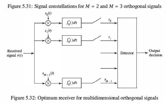
Optimum Receiver for the AWGN Channel
The receiver that minimizes the probability of error first passes the signal r(t) through
a parallel bank of M matched filters or M correlators. Because the signal correlators
and matched filters yield the same output at the sampling instant, let us consider the
case in which signal correlators are used, as shown in Figure 5.32.
Signal Correlators
The Detector
Matlab Coding
1 % MATLAB script M = 4 orthogonal signals for Monte Carlo simulation
 2 echo on
 3 clear;
 4 SNRindB=0:2:10;
 5 for i=1:length(SNRindB),
 6     % simulated error rate
 7     smld_err_prb(i)=smldP510(SNRindB(i));
 8     echo off;
 9 end;
M = 4;
for i=1:length(SNRindB_T)
SNR=exp(SNRindB_T(i)*log(10)/10);
% theoretical error rate
theo_err_prb(i)= (2*(M-1)/M)*Qfunct(sqrt((6*log2(M)/(M^2-1))*SNR));
echo off ;
end
10 echo on;
11 % Plotting commands follow
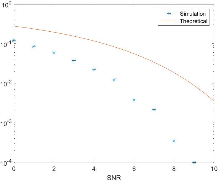
12 semilogy(SNRindB,smld_err_prb,‘*‘);
13
hold on
semilogy(SNRindB_T,theo_err_prb,‘-‘);
xlabel(‘SNR‘);
14
15 function [p]=smldP510(snr_in_dB)
16 % [p]=smldP510(snr_in_dB)
17 % SMLDP510 simulates the probability of error for the given
18 % snr_in_dB, signal-to-noise ratio in dB.
19 M=4; % quaternary orthogonal signaling
20 E=1;
21 SNR=exp(snr_in_dB*log(10)/10); % signal-to-noise ratio per bit
22 sgma=sqrt(E^2/(4*SNR)); % sigma, standard deviation of noise
23 N=10000; % number of symbols being simulated
24 % generation of the quaternary data source
25 for i=1:N,
26 temp=rand; % a uniform random variable over (0,1)
27 if (temp<0.25),
28 dsource1(i)=0;
29 dsource2(i)=0;
30 elseif (temp<0.5),
31 dsource1(i)=0;
32 dsource2(i)=1;
33 elseif (temp<0.75),
34 dsource1(i)=1;
35 dsource2(i)=0;
36 else
37 dsource1(i)=1;
38 dsource2(i)=1;
39 end
40 end;
41 % detection, and probability of error calculation
42 numoferr=0;
43 for i=1:N,
44 % matched filter outputs
45 if ((dsource1(i)==0) & (dsource2(i)==0)),
46 r0=sqrt(E)+gngauss(sgma);
47 r1=gngauss(sgma);
48 r2=gngauss(sgma);
49 r3=gngauss(sgma);
50 elseif ((dsource1(i)==0) & (dsource2(i)==1)),
51 r0=gngauss(sgma);
52 r1=sqrt(E)+gngauss(sgma);
53 r2=gngauss(sgma);
54 r3=gngauss(sgma);
55 elseif ((dsource1(i)==1) & (dsource2(i)==0)),
56 r0=gngauss(sgma);
57 r1=gngauss(sgma);
58 r2=sqrt(E)+gngauss(sgma);
59 r3=gngauss(sgma);
60 else
61 r0=gngauss(sgma);
62 r1=gngauss(sgma);
63 r2=gngauss(sgma);
64 r3=sqrt(E)+gngauss(sgma);
65 end;
66 % the detector
67 max_r=max([r0 r1 r2 r3]);
68 if (r0==max_r),
69 decis1=0;
70 decis2=0;
71 elseif (r1==max_r),
72 decis1=0;
73 decis2=1;
74 elseif (r2==max_r),
75 decis1=1;
76 decis2=0;
77 else
78 decis1=1;
79 decis2=1;
80 end;
81 % Count the number of bit errors made in this decision.
82 if (decis1~=dsource1(i)), % If it is an error, increase the error counter.
83 numoferr=numoferr+1;
84 end;
85 if (decis2~=dsource2(i)), % If it is an error, increase the error counter.
86 numoferr=numoferr+1;
87 end;
88 end;
89 p=numoferr/(2*N); % bit error probability estimate
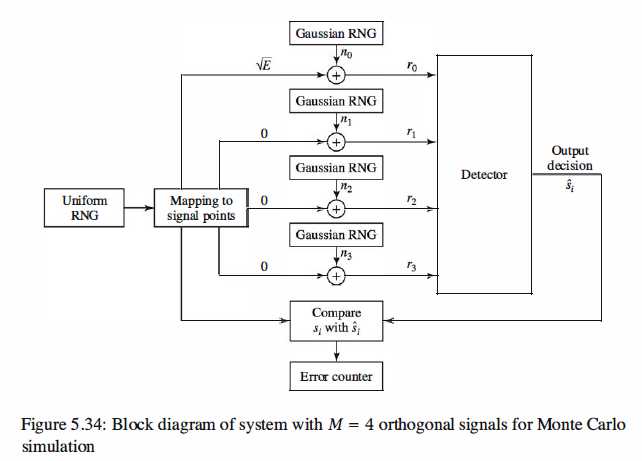
Simulation Result
Reference,
1. <<Contemporary Communication System using MATLAB>> - John G. Proakis
原文:https://www.cnblogs.com/zzyzz/p/13649081.html