Using Python to realize difference method. Here the data is from expermient. Use Central Difference method to solve the inner points, while forward difference for left and bottom boundary, backward difference for right and top boundary.

1 import numpy as np
2 import matplotlib.pyplot as plt
3 import matplotlib.mlab as mlab
1 data_vertex = np.loadtxt(‘Velocity0241.dat‘, dtype=float, delimiter=‘,‘, skiprows=1)
2 #data_vertex = np.genfromtxt(‘Velocity0241.dat‘, dtype=float, delimiter=‘,‘,skip_header=1)
3
4 print(len(data_vertex))
5
6 X = data_vertex[:,0]
7 Y = data_vertex[:,1]
8 U = data_vertex[:,2]
9 V = data_vertex[:,3]
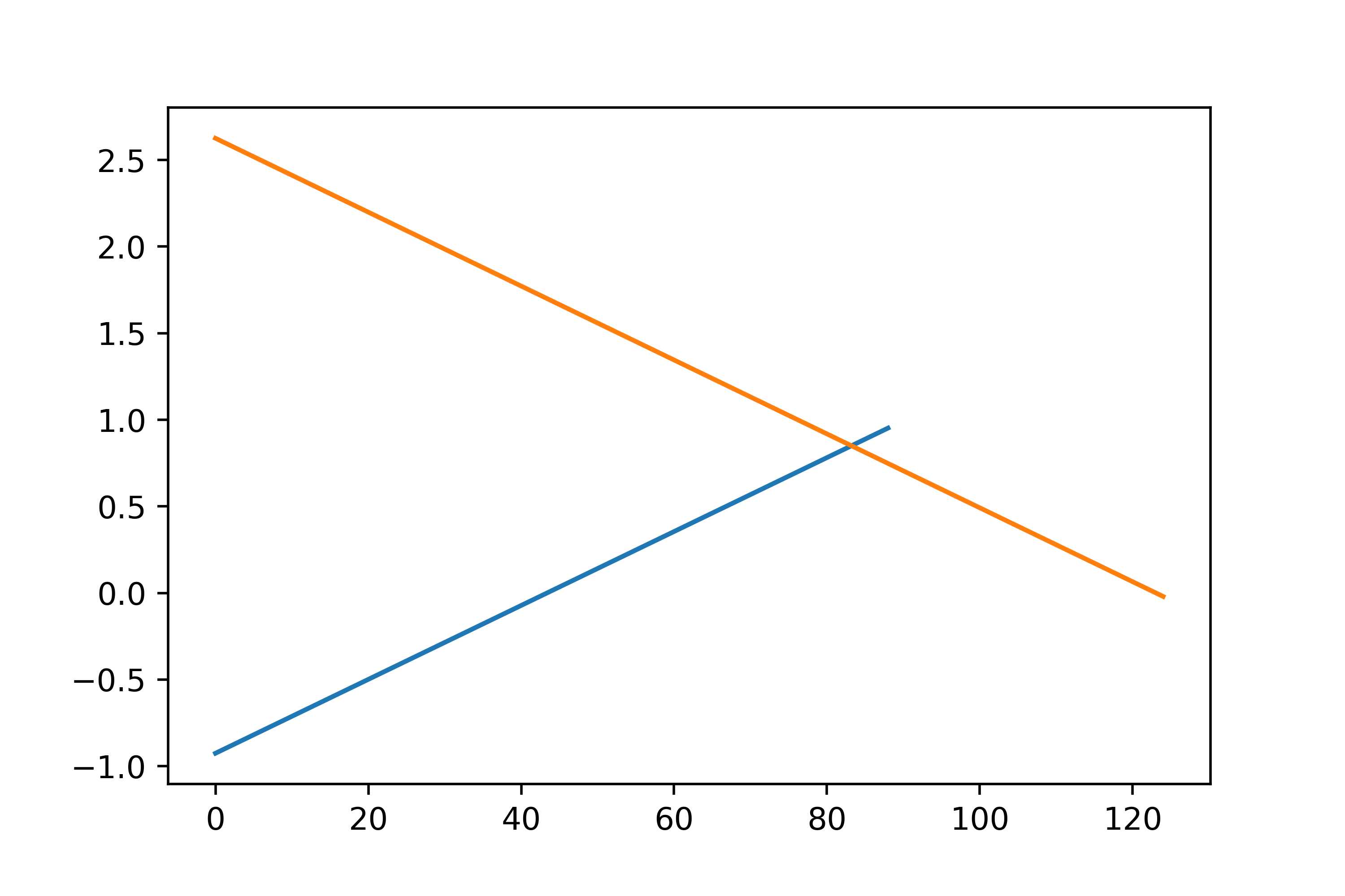
 1 ‘‘‘
 2 x = X.reshape(89,125)
 3 y = Y.reshape(89,125)
 4 u = U.reshape(89,125)
 5 v = V.reshape(89,125)
 6 ‘‘‘
 7
 8 x = np.reshape(X,(89,125))
 9 y = np.reshape(Y,(89,125))
10 u = np.reshape(U,(89,125))
11 v = np.reshape(V,(89,125))
12
13 num_row = x.shape[0]    # get number of rows of Mc
14 num_colume =y.shape[1] # get number of columes of Mc
15
16 print(num_row)
17 print(num_colume)
18
19 print(np.shape(x))
20 print(y[0,:])
21
22
23
24 plt.plot(x[:,0])
25 plt.plot(y[0,:])
26
27 plt.savefig(‘space_linear.png‘, dpi=500)
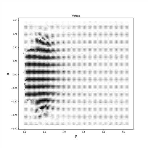
 1 # streamplot
 2
 3 import numpy as np
 4 import matplotlib.pyplot as plt
 5 import matplotlib.mlab as mlab
 6
 7
 8 fig, ax = plt.subplots(figsize=(10,10))
 9 ax.quiver(y,x,v,u)
10 #ax.quiver(y,x,v,u,color=‘red‘, width=0.005, scale=50)
11
12 ax.set_title(‘Vortex‘)
13 ax.set_xlabel(‘y‘,size=20)
14 plt.ylabel(‘x‘,size=20)
15
16 plt.savefig(‘vector_field_of_velocity.png‘,dpi=200,format=‘png‘)
17
18 plt.show()
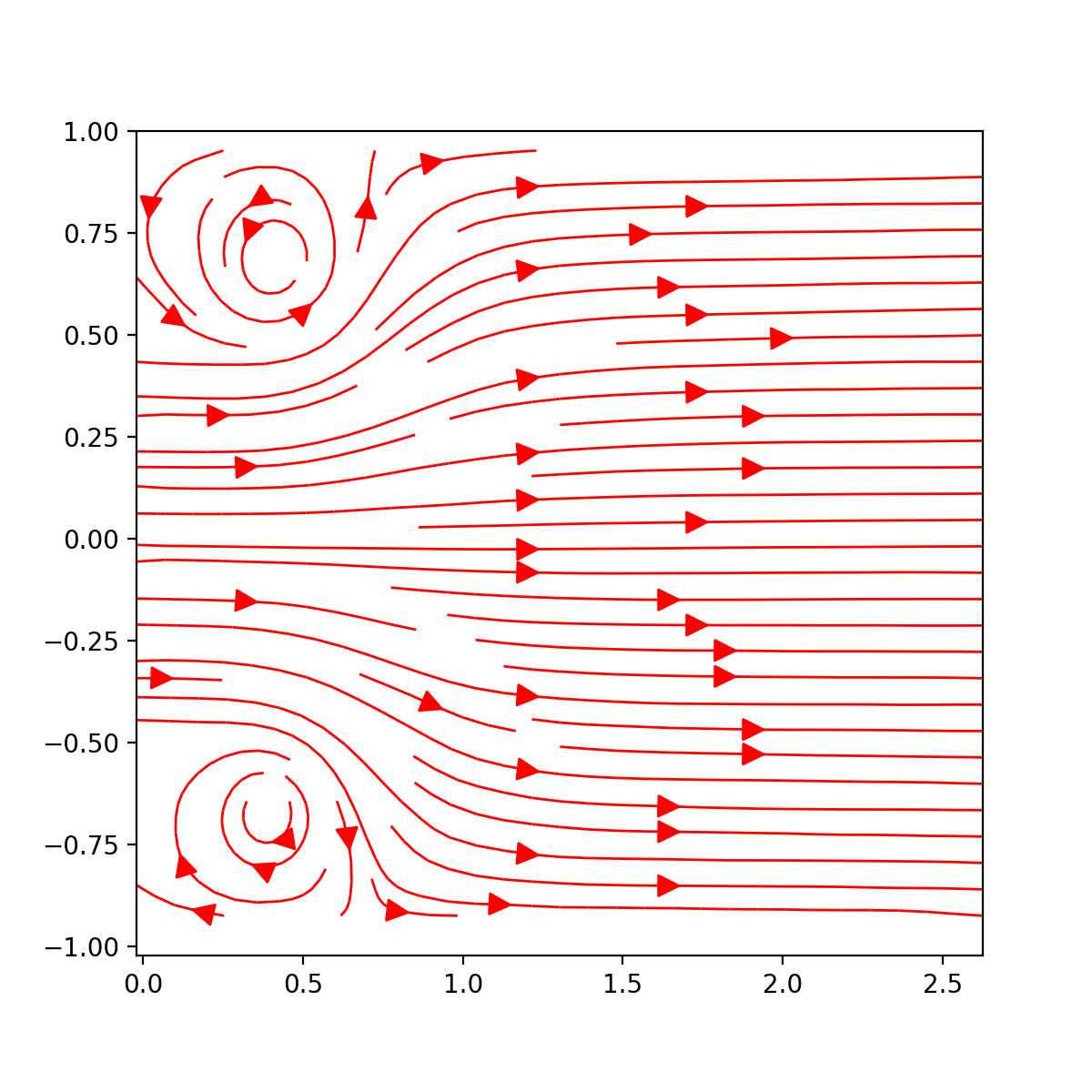
 1 # streamplot
 2
 3 import numpy as np
 4 import matplotlib.pyplot as plt
 5 import matplotlib.mlab as mlab
 6
 7 fig, ax = plt.subplots(figsize=(6,6))
 8
 9 x1 = np.linspace(x[0][0],x[88][0],89)
10 y1 = np.linspace(y[0][0],y[0][124],125)
11
12 ax.streamplot(y1,x1,v,u,13  density=1, linewidth=1, color=‘r‘, arrowsize=2)
14
15 ax.yaxis.set_ticks([-1.0,-0.75,-0.5,-0.25,0.0,0.25,0.5,0.75,1.0])
16
17 plt.savefig(‘vortics.png‘,dpi=200,format=‘png‘)
18
19 plt.show()
20
21
22 ‘‘‘
23 fig = plt.figure()
24 ax = fig.gca() # gca get current axis
25 ax.streamplot(y,x,v,u)
26 ‘‘‘
 1 # gradient function in x direction
 2 def dx(M, space): # dx:derivative x
 3     Mc = M.copy()
 4     num_row = Mc.shape[0]    # get number of rows of Mc
 5     num_colume = Mc.shape[1] # get number of columes of Mc
 6     for i in range(num_row):
 7         for j in range(num_colume):
 8             if i == 0:   # left boundary, we use forward difference method
 9                 Mc[i][j] = (M[i+1][j] - M[i][j]) / (space)
10             elif i == (num_row - 1):  # right boundary, we use backward difference method
11                 Mc[i][j] = (M[i][j] - M[i-1][j]) / (space)
12
13             else:   # inner points, we use central difference method
14                 Mc[i][j] = (M[i+1][j] - M[i-1][j]) / (2*space)
15     return Mc
16
17 # gradient function in y direction
18 def dy(M,space):
19     Mc = M.copy()
20     for i in range(num_row):
21         for j in range(num_colume):
22             if j == 0:   # lower boundary, use forward difference
23                 Mc[i][j] = (M[i][j+1] - M[i][j]) / (space)
24             elif j == (num_colume - 1):   #upper boundary, use backward fifference
25                 Mc[i][j] = (M[i][j] - M[i][j-1]) / (space)
26             else:   # inner points, use central difference
27                 Mc[i][j] = (M[i][j+1] - M[i][j-1]) / (2*space)
28     return Mc
29
30 delta_x = x[1][0] - x[0][0]
31 delta_y = y[0][1] - y[0][0]
32
33 dudx = dx(u, delta_x)
34 dudy = dy(u, delta_y)
35 dvdx = dx(v, delta_x)
36 dvdy = dy(v, delta_y)
37
38 print(delta_x)
39 print(delta_y)
1 Div = np.array(dudx) + np.array(dvdy)
2
3 Curl = np.array(dvdx) - np.array(dudy)
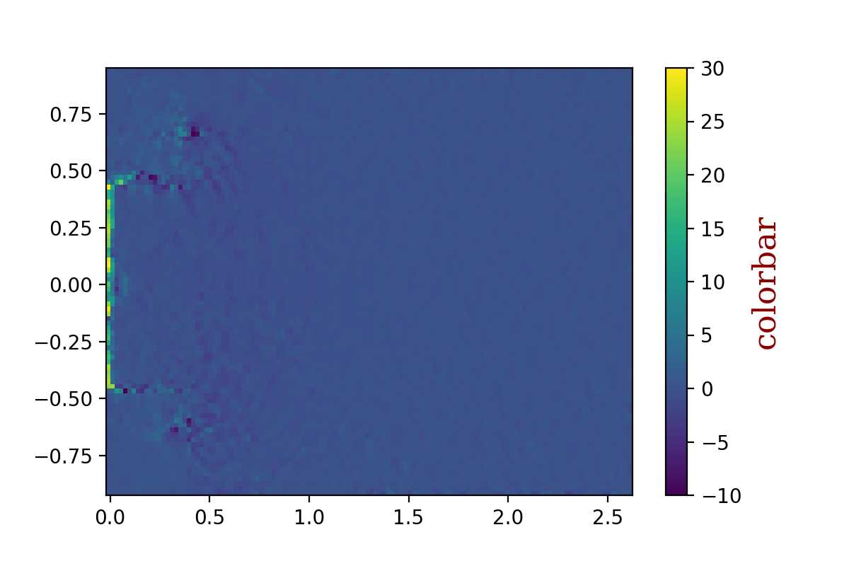
 1 import numpy as np
 2 import matplotlib.pyplot as plt
 3
 4 print(np.shape(Div))
 5
 6 p = plt.pcolormesh(y,x,Div,vmin=-10, vmax=30)
 7
 8 cb = plt.colorbar(p)
 9 cb.ax.tick_params(labelsize=10)
10
11 font = {‘family‘ : ‘serif‘,
12         ‘color‘  : ‘darkred‘,
13         ‘weight‘ : ‘normal‘,
14         ‘size‘   : 16,
15         }
16 cb.set_label(‘colorbar‘,fontdict=font)
17
18 #cb.ax.tick_params(labelsize=32)
19
20 plt.savefig(‘divergence.png‘,dpi=200)
21
22 plt.xticks(fontsize=16)
23 plt.yticks(fontsize=8)
24 plt.show()
25
26 ‘‘‘
27 divergence should be 0 for incompressible flow according to fluid mechanics, but here
28 it is not 0, that might because the real flow is 3D, but here we just calculate 2d,
29 in xy plane, and ignore the contribution of the third dimension to divergence
30 ‘‘‘
 1 import numpy as np
 2 import matplotlib.pyplot as plt
 3
 4 print(np.shape(Curl))
 5
 6 p = plt.pcolormesh(y,x,Curl) # The rotation is in the opposite direction
 7
 8 plt.colorbar(p)
 9
10 plt.savefig(‘curl.png‘,dpi=200)
11
12 plt.show()
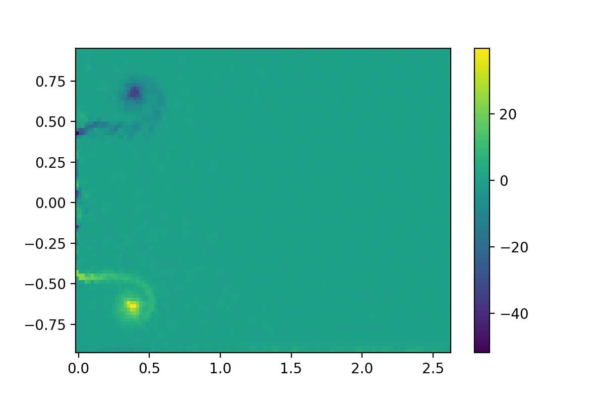
Python: use central difference method to solve curl equation and plot it
原文:https://www.cnblogs.com/cfdchen/p/13759947.html