Calculating Moving Average in R

1. Introduction

I am surprised there are some high level functions shipped with R base, like download.file(). However, I am even more surprised there is no built in moving average function in R, as it is known as statistical analysis software.

The first article on moving average in R I found was in 2012, but until today there is still no such function for users. Maybe the community feel it is too old to care about, or as if they are real minimalists (and somehow they suddenly feel not like being minimalists when building download.file()).

Nevertheless this is an article about how to do moving average or rolling mean in R in 2020-Oct.

2. Preparation

library(tidyverse)
library(lubridate)
library(nycflights13)

I would like to use tidyverse for data transforming, lubridate for dealing with date and time data, and nycflights13 as data set.

So we import they at the beginning.

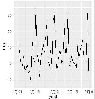
daily <- flights %>%
  mutate(ymd = make_date(year, month, day)) %>%
  filter(month<=2) %>%
  group_by(ymd) %>%
  summarise(mean = mean(arr_delay, na.rm=TRUE))
daily

ggplot(data=daily) +
  geom_line(aes(x=ymd, y=mean))

I simply import nycflights13::flights and add new column named "ymd". This column is build by lubridate::make_date() from existing columns "year", "month", "day".

After that, I filter only Jan and Feb data for convenience. Group by "ymd" column. Finally summarise with mean of "arr_delay" column.

This is how daily looks like and the plot for it.

# A tibble: 59 x 2
   ymd          mean
   <date>      <dbl>
 1 2013-01-01 12.7  
 2 2013-01-02 12.7  
 3 2013-01-03  5.73 
 4 2013-01-04 -1.93 
 5 2013-01-05 -1.53 
 6 2013-01-06  4.24 
 7 2013-01-07 -4.95 
 8 2013-01-08 -3.23 
 9 2013-01-09 -0.264
10 2013-01-10 -5.90 
# ... with 49 more rows

3. Method One, Using stats::filter()

Warning: there is a built in filter() function with R. But if we use tidyverse or dplyr at the same time, their filter() function will overwrite the default one. So make sure to use stats::filter().

mav <- function(x, n) {
  stats::filter(x, rep(1/n, n), side=1)
}

example1 <- daily %>%
  mutate(mav7 = mav(mean, 7),
         mav14 = mav(mean, 14))
example1

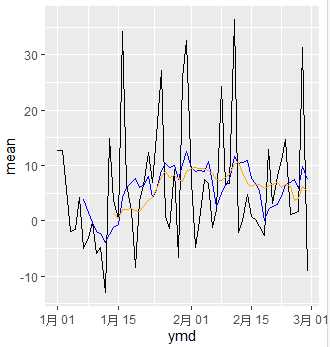
ggplot(data=example1) +
  geom_line(aes(x=ymd, y=mean), color="black") +
  geom_line(aes(x=ymd, y=mav7), color="blue") +
  geom_line(aes(x=ymd, y=mav14), color="orange")

stats::filter() function has a bad name becuase it doesn‘t actually do filter job like we expected. (This is one reason explains why old version R is not good enough and why we need tidyverse today.)

stats::filter() distributes coefficients to our vector x and do cumsum summary.  rep(1/n, n) means create a collection with n numbers of 1/n. 

So stats::filter() distributes 1/n to each member of x and do cumsum summary.

This is exactly what we need in moving average. So we wrapped it up as a moving average function.

Argument side= is set to 1. This contorls two styles of moving average. side=1 or side=2.

> example1
# A tibble: 59 x 4
   ymd          mean   mav7 mav14
   <date>      <dbl>  <dbl> <dbl>
 1 2013-01-01 12.7   NA        NA
 2 2013-01-02 12.7   NA        NA
 3 2013-01-03  5.73  NA        NA
 4 2013-01-04 -1.93  NA        NA
 5 2013-01-05 -1.53  NA        NA
 6 2013-01-06  4.24  NA        NA
 7 2013-01-07 -4.95   3.84     NA
 8 2013-01-08 -3.23   1.58     NA
 9 2013-01-09 -0.264 -0.275    NA
10 2013-01-10 -5.90  -1.94     NA
# ... with 49 more rows

4. Method Two, Using zoo::rollmean()

This library zoo is not in the landscape of tidyverse. It works with date and time data like lubridate.

It has a clear function called rollmean() to do moving average(roll mean).

library(zoo)
example2 <- daily %>%
  mutate(mav7 = rollmean(mean, 7, na.pad=TRUE, align="right"),
         mav14 = rollmean(mean, 14, na.pad=TRUE, align="right"))
example2

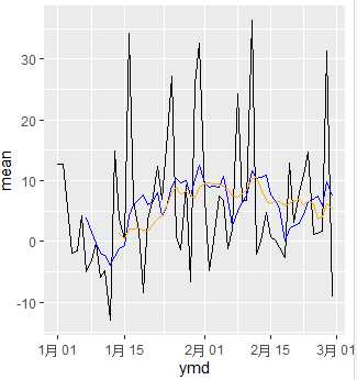
ggplot(data=example2) +
  geom_line(aes(x=ymd, y=mean), color="black") +
  geom_line(aes(x=ymd, y=mav7), color="blue") +
  geom_line(aes(x=ymd, y=mav14), color="orange")

Two things should be noticed in zoo::rollmean().

First, na.pad=TRUE should be used, otherwise the output vector lenght will not be the same as input vector. This will stop us create new column data transforming.

Second, align= should be used. It can be chosen as "left", "center", or "right". It means different style of moving average.

> example2
# A tibble: 59 x 4
   ymd          mean   mav7 mav14
   <date>      <dbl>  <dbl> <dbl>
 1 2013-01-01 12.7   NA        NA
 2 2013-01-02 12.7   NA        NA
 3 2013-01-03  5.73  NA        NA
 4 2013-01-04 -1.93  NA        NA
 5 2013-01-05 -1.53  NA        NA
 6 2013-01-06  4.24  NA        NA
 7 2013-01-07 -4.95   3.84     NA
 8 2013-01-08 -3.23   1.58     NA
 9 2013-01-09 -0.264 -0.275    NA
10 2013-01-10 -5.90  -1.94     NA
# ... with 49 more rows

5. A Little Check

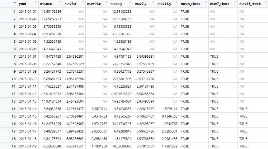
check <- merge(example1, example2, by=‘ymd‘) %>% 
  as_tibble() %>% 
  mutate(mean_check = near(mean.x, mean.y),
         mav7_check=near(mav7.x, mav7.y),
         mav14_check=near(mav14.x, mav14.y))

For clearly see these two methods result the same, I do a little check.

We use near() instead of "== ", because they are float points numbers so they may not be exactly the same in logic "==". 

Calculating Moving Average in R

原文：https://www.cnblogs.com/drvongoosewing/p/13905502.html