https://scikit-learn.org/stable/tutorial/statistical_inference/putting_together.html#pipelining
有的模型用于转换数据, 有的模型用于预测数据。
可以将这两种模型组合起来, 这就是流水线技术。
如下面的例子, 是将PCA分解 和 回归学习, 组合成一个新的模型。
We have seen that some estimators can transform data and that some estimators can predict variables. We can also create combined estimators:
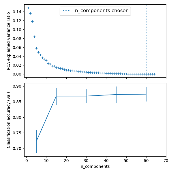
import numpy as np
import matplotlib.pyplot as plt
import pandas as pd

from sklearn import datasets
from sklearn.decomposition import PCA
from sklearn.linear_model import LogisticRegression
from sklearn.pipeline import Pipeline
from sklearn.model_selection import GridSearchCV


# Define a pipeline to search for the best combination of PCA truncation
# and classifier regularization.
pca = PCA()
# set the tolerance to a large value to make the example faster
logistic = LogisticRegression(max_iter=10000, tol=0.1)
pipe = Pipeline(steps=[(‘pca‘, pca), (‘logistic‘, logistic)])

X_digits, y_digits = datasets.load_digits(return_X_y=True)

# Parameters of pipelines can be set using ‘__’ separated parameter names:
param_grid = {
    ‘pca__n_components‘: [5, 15, 30, 45, 64],
    ‘logistic__C‘: np.logspace(-4, 4, 4),
}
search = GridSearchCV(pipe, param_grid, n_jobs=-1)
search.fit(X_digits, y_digits)
print("Best parameter (CV score=%0.3f):" % search.best_score_)
print(search.best_params_)

# Plot the PCA spectrum
pca.fit(X_digits)

fig, (ax0, ax1) = plt.subplots(nrows=2, sharex=True, figsize=(6, 6))
ax0.plot(np.arange(1, pca.n_components_ + 1),
         pca.explained_variance_ratio_, ‘+‘, linewidth=2)
ax0.set_ylabel(‘PCA explained variance ratio‘)

ax0.axvline(search.best_estimator_.named_steps[‘pca‘].n_components,
            linestyle=‘:‘, label=‘n_components chosen‘)
ax0.legend(prop=dict(size=12))
https://scikit-learn.org/stable/auto_examples/compose/plot_digits_pipe.html
The PCA does an unsupervised dimensionality reduction, while the logistic regression does the prediction.
We use a GridSearchCV to set the dimensionality of the PCA
Out:
Best parameter (CV score=0.920):
{‘logistic__C‘: 0.046415888336127774, ‘pca__n_components‘: 45}
https://scikit-learn.org/stable/tutorial/statistical_inference/putting_together.html#face-recognition-with-eigenfaces
本例是使用 SVM 模型来 预测 人脸的对应的是谁。
首先使用PCA提取 不同尺度的特征, 然后使用SVM 去学习特征和人名之间的关系。
The dataset used in this example is a preprocessed excerpt of the “Labeled Faces in the Wild”, also known as LFW:
"""
===================================================
Faces recognition example using eigenfaces and SVMs
===================================================

The dataset used in this example is a preprocessed excerpt of the
"Labeled Faces in the Wild", aka LFW_:

  http://vis-www.cs.umass.edu/lfw/lfw-funneled.tgz (233MB)

.. _LFW: http://vis-www.cs.umass.edu/lfw/

Expected results for the top 5 most represented people in the dataset:

================== ============ ======= ========== =======
                   precision    recall  f1-score   support
================== ============ ======= ========== =======
     Ariel Sharon       0.67      0.92      0.77        13
     Colin Powell       0.75      0.78      0.76        60
  Donald Rumsfeld       0.78      0.67      0.72        27
    George W Bush       0.86      0.86      0.86       146
Gerhard Schroeder       0.76      0.76      0.76        25
      Hugo Chavez       0.67      0.67      0.67        15
       Tony Blair       0.81      0.69      0.75        36

      avg / total       0.80      0.80      0.80       322
================== ============ ======= ========== =======

"""
from time import time
import logging
import matplotlib.pyplot as plt

from sklearn.model_selection import train_test_split
from sklearn.model_selection import GridSearchCV
from sklearn.datasets import fetch_lfw_people
from sklearn.metrics import classification_report
from sklearn.metrics import confusion_matrix
from sklearn.decomposition import PCA
from sklearn.svm import SVC


print(__doc__)

# Display progress logs on stdout
logging.basicConfig(level=logging.INFO, format=‘%(asctime)s %(message)s‘)


# #############################################################################
# Download the data, if not already on disk and load it as numpy arrays

lfw_people = fetch_lfw_people(min_faces_per_person=70, resize=0.4)

# introspect the images arrays to find the shapes (for plotting)
n_samples, h, w = lfw_people.images.shape

# for machine learning we use the 2 data directly (as relative pixel
# positions info is ignored by this model)
X = lfw_people.data
n_features = X.shape[1]

# the label to predict is the id of the person
y = lfw_people.target
target_names = lfw_people.target_names
n_classes = target_names.shape[0]

print("Total dataset size:")
print("n_samples: %d" % n_samples)
print("n_features: %d" % n_features)
print("n_classes: %d" % n_classes)


# #############################################################################
# Split into a training set and a test set using a stratified k fold

# split into a training and testing set
X_train, X_test, y_train, y_test = train_test_split(
    X, y, test_size=0.25, random_state=42)


# #############################################################################
# Compute a PCA (eigenfaces) on the face dataset (treated as unlabeled
# dataset): unsupervised feature extraction / dimensionality reduction
n_components = 150

print("Extracting the top %d eigenfaces from %d faces"
      % (n_components, X_train.shape[0]))
t0 = time()
pca = PCA(n_components=n_components, svd_solver=‘randomized‘,
          whiten=True).fit(X_train)
print("done in %0.3fs" % (time() - t0))

eigenfaces = pca.components_.reshape((n_components, h, w))

print("Projecting the input data on the eigenfaces orthonormal basis")
t0 = time()
X_train_pca = pca.transform(X_train)
X_test_pca = pca.transform(X_test)
print("done in %0.3fs" % (time() - t0))


# #############################################################################
# Train a SVM classification model

print("Fitting the classifier to the training set")
t0 = time()
param_grid = {‘C‘: [1e3, 5e3, 1e4, 5e4, 1e5],
              ‘gamma‘: [0.0001, 0.0005, 0.001, 0.005, 0.01, 0.1], }
clf = GridSearchCV(
    SVC(kernel=‘rbf‘, class_weight=‘balanced‘), param_grid
)
clf = clf.fit(X_train_pca, y_train)
print("done in %0.3fs" % (time() - t0))
print("Best estimator found by grid search:")
print(clf.best_estimator_)


# #############################################################################
# Quantitative evaluation of the model quality on the test set

print("Predicting people‘s names on the test set")
t0 = time()
y_pred = clf.predict(X_test_pca)
print("done in %0.3fs" % (time() - t0))

print(classification_report(y_test, y_pred, target_names=target_names))
print(confusion_matrix(y_test, y_pred, labels=range(n_classes)))


# #############################################################################
# Qualitative evaluation of the predictions using matplotlib

def plot_gallery(images, titles, h, w, n_row=3, n_col=4):
    """Helper function to plot a gallery of portraits"""
    plt.figure(figsize=(1.8 * n_col, 2.4 * n_row))
    plt.subplots_adjust(bottom=0, left=.01, right=.99, top=.90, hspace=.35)
    for i in range(n_row * n_col):
        plt.subplot(n_row, n_col, i + 1)
        plt.imshow(images[i].reshape((h, w)), cmap=plt.cm.gray)
        plt.title(titles[i], size=12)
        plt.xticks(())
        plt.yticks(())


# plot the result of the prediction on a portion of the test set

def title(y_pred, y_test, target_names, i):
    pred_name = target_names[y_pred[i]].rsplit(‘ ‘, 1)[-1]
    true_name = target_names[y_test[i]].rsplit(‘ ‘, 1)[-1]
    return ‘predicted: %s\ntrue:      %s‘ % (pred_name, true_name)

prediction_titles = [title(y_pred, y_test, target_names, i)
                     for i in range(y_pred.shape[0])]

plot_gallery(X_test, prediction_titles, h, w)

# plot the gallery of the most significative eigenfaces

eigenface_titles = ["eigenface %d" % i for i in range(eigenfaces.shape[0])]
plot_gallery(eigenfaces, eigenface_titles, h, w)

plt.show()
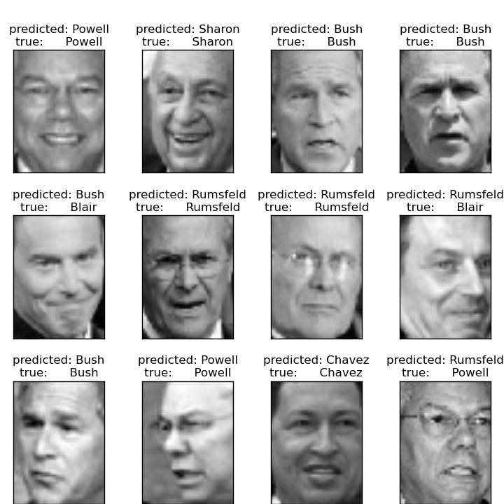
Prediction
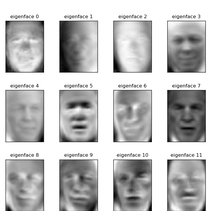
Eigenfaces
Expected results for the top 5 most represented people in the dataset:
                   precision    recall  f1-score   support

Gerhard_Schroeder       0.91      0.75      0.82        28
  Donald_Rumsfeld       0.84      0.82      0.83        33
       Tony_Blair       0.65      0.82      0.73        34
     Colin_Powell       0.78      0.88      0.83        58
    George_W_Bush       0.93      0.86      0.90       129

      avg / total       0.86      0.84      0.85       282
https://scikit-learn.org/stable/tutorial/statistical_inference/putting_together.html#open-problem-stock-market-structure
Can we predict the variation in stock prices for Google over a given time frame?
https://scikit-learn.org/stable/auto_examples/applications/plot_stock_market.html#stock-market
This example employs several unsupervised learning techniques to extract the stock market structure from variations in historical quotes.
The quantity that we use is the daily variation in quote price: quotes that are linked tend to cofluctuate during a day.
statistical learning -- putting_together of sklearn
原文:https://www.cnblogs.com/lightsong/p/14227621.html