论文链接:https://www.aclweb.org/anthology/2020.acl-main.141/
代码链接(Pytorch):https://github.com/nanguoshun/LSR
这篇我个人感觉是EoG模型的改良,针对的问题就是:在EoG模型的消融实验中,发现full version在长度大于4时的效果要比原始的EoG模型要好,那么在full的情况下,是否可以让模型自动选择哪些边重要,那些不重要呢?这就是LSR模型。
1 Introduction
Peng et al. (2017) construct dependency graph to capture interactions among n-ary entities for cross-sentence extraction.
Sahu et al. (2019) extend this approach by using co-reference links to connect dependency trees of sentences to construct the document-level graph.
Instead, Christopoulou et al. (2019) construct a heterogeneous graph based on a set of heuristics, and then apply an edge-oriented model (Christopoulou et al., 2018) to perform inference.
与以前的文档级结构由共同引用和规则构成constructed by co-references and rules方法不同,我们提出的模型将图结构视为一个潜在变量latent variable,并以端到端的方式进行归纳。Our model is built based on the structured attention (Kim et al., 2017; Liu and Lapata, 2018). Using a variant of Matrix-Tree Theorem【TODO】 (Tutte, 1984; Koo et al., 2007),我们的模型能够生成特定于任务的依赖结构来捕获实体之间的非局部交互。我们进一步开发了一种迭代细化策略iterative refinement strategy,使我们的模型能够基于上一次迭代动态构建潜在结构latent structure,从而使模型能够增量捕获复杂的交互,从而实现更好的多跳推理multi-hop reasoning(Welbl et al.,2018)
实验表明,我们的模型在DocRED(一个包含大量实体和关系的大规模文档级关系抽取数据集)上的性能明显优于现有的方法,并在生物医学领域两个流行的文档级关系抽取数据集上得到了最新的结果。我们的贡献总结如下:
1.我们以端到端的方式构造文档级图进行推理,而不依赖于共同引用或规则without relying on co-references or rules,这可能并不总是产生最优结构。通过迭代求精策略,我们的模型能够动态地构造一个潜在的结构来改进整个文档中的信息聚合。
2.我们进行定量和定性分析,与各种环境下的最先进模型进行比较。我们证明,利用多跳推理模块我们的模型能够发现更准确的句间关系。
2 Model
Our LSR model consists of three components: node constructor, dynamic reasoner, and classifier.
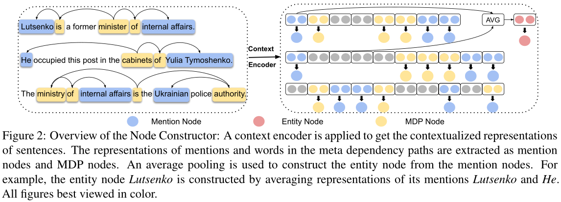
The node constructor first encodes each sentence of an input document and outputs contextual representations.Representations that correspond to mentions and tokens on the shortest dependency path in a sentence are extracted as nodes.对应于句子中最短依赖路径上的提及和标记的表示被提取为节点。
The dynamic reasoner is then applied to induce a document-level structure based on the extracted nodes.然后应用动态推理器,根据提取的节点归纳出文档级结构。Representations of nodes are updated based on information propagation on the latent structure, which is iteratively refined.基于潜在结构上的信息传播更新节点表示,并对其进行迭代细化。
Final representations of nodes are used to calculate classification scores by the classifier.
2.1 Node Constructor
节点构造器将文档中的句子编码为上下文表示,并构造提及节点、实体节点和元依赖路径(MDP)节点mention nodes, entity nodes and meta dependency paths (MDP) nodes的表示,如图2所示。这里MDP表示一个句子中所有提及的一组最短依赖路径,MDP中的令牌被提取为MDP节点。Here MDP indicates a set of shortest dependency paths for all mentions in a sentence, and tokens in the MDP are extracted as MDP nodes.
这一部分分为两小部分:context encoding与node extraction,主要就是对document中的所有word进行编码,并得到graph所有类型的node的representation
Context encoding:对于给定的document $d$,我们将其输入到一个encoder中(BILSTM/BERT etc),得到contextual representation。
node extraction:在LSR中,有三种node:mention node、entity node以及meta dependancy path node。mention node表示的是一个sentence中entity的所有的mention,其表示是该mention中的所有word的representation的平均;entity node指的是entity node,其表示是所有mention node的representation的平均;MDP表示一个句子中所有mention的最短依赖路径集,在MDP元依赖路径中,mention和单词的表示分别被提取为提及节点和MDP节点。
??LSR与EoG模型不同的地方之一在于:mention node与entity node一样的,但是LSR没有sentence node,并且使用了MDP node来代替,本质上差不多吧,不过相比于sentence node,MDP node能够过滤掉无关信息(paper原话??),但是说实话,在context encoding中,已经引入了无关信息吧,而且在之后的实验中,确实也证明MDP没啥用。
2.2 Dynamic Reasoner
这一部分就是inference,因为在EoG里面,已经证明了没有inference对最终结果影响还是蛮大的。主要分为两部分:structure induction与multi-hop reasioning。
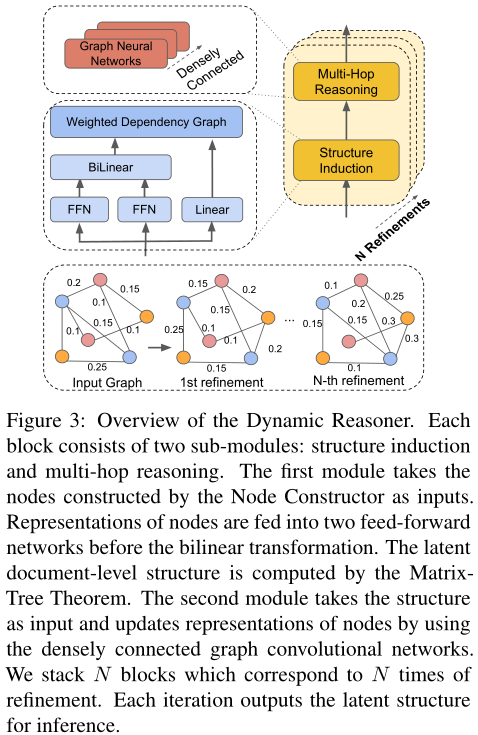
图3:动态推理器的概述。每个模块包括两个子模块:结构归纳和多跳推理。第一个模块将节点构造函数构造的节点作为输入。在双线性变换之前,节点的表示被馈送到两个前馈网络中。利用矩阵树定理计算文档的潜在层次结构。第二个模块以结构为输入,利用密接图卷积网络更新节点表示。我们叠加N个块,对应N次细化。每次迭代都会输出潜在的结构进行推理。
2.2.1 Structure Induction
与现有的使用共同引用链接(Sahu et al.,2019)或启发式(Christopoulou et al.,2019)来构建文档级图进行推理的模型不同,我们的模型将图形视为一个潜在变量,并以端到端的方式进行归纳。结构诱导模块是基于结构化注意the structured attention构建的(Kim et al.,2017;Liu and Lapata,2018)。受Liu和Lapata(2018)的启发,我们使用Kirchhoff矩阵树定理Matrix-Tree Theorem的变体(Tutte,1984;Koo et al.,2007)来诱导潜在依赖结构。
Let $u_i$ denote the contextual representation of the i-th node, where $u_i∈ R^d$, we first calculate the pair-wise unnormalized attention score $s_{ij}$ between the i-th and the j-th node with the node representations $u_i$ and $u_j$.The score $s_{ij} is calculated by two feed-forward neural networks and a bilinear transformation:
$s_{ij}=(tanh(W_pu_i))^TW_b(tanh(W_cu_j))$
where $W_p∈ R^{d×d}$ and $W_c∈ R^{d×d}$ are weights for two feed-forward neural networks, $d$ is the dimension of the node representations, and $tanh$ is applied as the activation function. $W_b∈ R^{d×d}$ are the weights for the bilinear transformation.Next we compute the root score $s_r$ iwhich represents the unnormalized probability of the i-th node to be selected as the root node of the structure:
$s_i^r=W_r^u_i$
where $W_r∈ R^{1×d}$ is the weight for the linear transformation线性变换.Following Koo et al. (2007), we calculate the marginal probability of each dependency edge of the document-level graph.For a graph G with n nodes, we first assign non-negative weights $P ∈ R^{n×n}$ to the edges of the graph(首先对边的值赋非负值):
$P_{ij} = \left\{ \begin{array}{lr} 0 & : if i=j\\ exp(s_{ij}) & : otherwise \end{array} \right$(5)
where $P_{ij}$ is the weight of the edge between the i-th and the j-th node. $P_{ij}$表示的是node i与node j之间的edge的权重,除了自身为0外,这真的是一个全连接的矩阵(根据相似度和概率生成)。We then define the Laplacian matrix $L ∈ R^{n×n}$ of G in Equation (6)
先说一句,拉普拉斯矩阵的定义,$L=D-P$ 度矩阵 – 邻接矩阵), and its variant $\hat{L} ∈ R^{n×n}$ in Equation (7) for further computations (Koo et al., 2007).
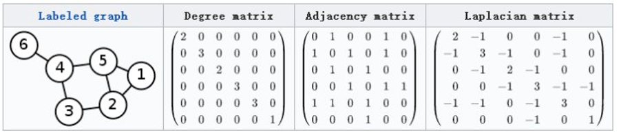
$L_{ij} = \left\{ \begin{array}{lr} \sum_{i^{‘}=1}^nP_{i^{‘}j} & : if i=j\\ -P_{ij} & : otherwise \end{array} \right$(6)
很好理解,就是把一个节点的边权相加,作为这个节点的度了嘛,下面就开始进入 Matrix-Tree Theorem知识范围了
$\hat{L_{ij}} = \left\{ \begin{array}{lr} exp(s_i^r) & : if i=1\\ L_{ij} & : if i>1 \end{array} \right$(7)
We use $A_{ij}$ to denote the marginal probability of the dependency edge between the i-th and the j-th node. Then, $A_{ij}$ can be derived based on Equation (8), where $\delta$ is the Kronecker delta (Koo et al., 2007).
$A_{ij}=(1-\delta_{1,j})P_{ij}[\hat{L}^{-1}]_{ij}-(1-\delta_{i,1})P_{ij}[\hat{L}^{-1}]_{ji}$
Here, $A ∈ R^{n×n}$ can be interpreted as a weighted adjacency matrix of the document-level entity graph. Finally, we can feed $A ∈ R^{n×n}$ into the multi-hop reasoning module to update the representations of nodes in the latent structure.
下面解释变异的拉普拉斯矩阵($\hat{L}$ is a variant of $L$ that takes the root node into consideration):
为什么要把第一行换成 root 的分数呢?(其实把任意一行换成 root 的分数都可以)这是因为在Matrix-Tree Theorem中计算一棵树的 logit 分数时,实际上是下面这个式子的形式(我简化了):
$\psi = r_{root}\prod P_{ij}$
很简单,就是这棵树根结点的分数乘以所有边的分数。那么在计算这个句子属于这棵树的概率时,就是:
$p=\frac{\psi}{\sum \psi}$
因此这里的分母$z = \sum(r_{root}\prod A_{ij})$。根据 Matrix-Tree Theorem,拉普拉斯矩阵的 minor$L^{(m,m)}$(就是矩阵的余子式的行列式)就等于以点 m 为根结点的所有生成树的权重之和,因此上面这个分母$z$可以用拉普拉斯矩阵表示:
$z=\sum(r_{root}L^{(m,m)})$
那这个式子不就是把$det(\hat{L})$按照第一行展开嘛!所以搞一个$\hat{L}$其实就是为了算$z$方便。$A_{ij}$的形成可以参考原文或者这篇博主:https://ivenwang.com/2020/12/29/structured/
2.2.2 Multi-hop Reasoning
在得到邻接矩阵之后,LSR便使用GCN来对graph进行aggregate。公式如下:
$u_i^l=\sigma(\sum_{j=1}^nA_{ij}W^lu_i^{l-1}+b^l)$(9)
$u^0_i∈ R^d$ is the initial contextual representation of the i-th node constructed by the node constructor.
我们使用到GCNs的密集连接,以便在大型文档级图上捕获更多的结构信息。在密集连接的帮助下,我们能够训练更深入的模型,从而能够捕获更丰富的局部和非局部信息,从而学习更好的图表示。每个图卷积层上的计算类似于等式(9)。这个密集连接的图网络和多头注意力机制的原理相似,而联想到图中边是根据两个节点经过注意力计算得到的,可以推测密集连接和多头注意力的效果相似,可以捕获图中不同的特征信息。
2.2.3 Iterative Refinement
上面用几层 GCN 更新 node 表示之后,再用这组 node 表示重新按 2.1 的步骤计算邻接矩阵,以此迭代循环。
为什么这样做呢?作者说,他看到 Matrix-Tree Theorem里面生成树都非常浅,觉得一次 structure induction 不能表示文档里复杂的结构,所以才要这样迭代多次。
2.3 Classifier
这一步就是直接对entity pair进行关系分类,使用sigmoid函数。如下:
$P(r|e_i,e_j)=\sigma(e_i^TW_ee_j+b_e)_r$
where $W_e∈ R^{d×k×d}$ and $b_e∈ R^k$ are trainable weights and bias, with $k$ being the number of relation categories, $sigma$ is the sigmoid function, and the subscript $r$ in the right side of the equation refers to the relation type.
3 Experiments
数据集:CDR、GDA、DocRED
Graph-based Models作为对比:
这些模型构建了任务特定的推理图。GCNN(Sahu et al.,2019)通过共同引用链接构建文档级图,然后应用关系GCN进行推理。
EoG(Christopoulou eta al,2019)是生物医学领域最先进的文档级关系抽取模型。EoG首先使用启发式方法构造图,然后利用面向边的模型进行推理。
GCNN和EoG是基于静态结构的。GAT(Veliˇckovi′c et al,2018)能够基于局部注意机制学习加权图结构。
AGGCN(Guo et al,2019a)是一种最新的句子级关系抽取模型,它通过自我注意来构建潜在结构。这两个模型能够动态地构造特定于任务的结构
BERT-based Models作为对比:
这些模型对DocRED的BERT(Devlin et al.,2019)进行了微调。具体而言,两阶段的BERT(Wang et al.,2019)是最好的report模型。它是一个管道模型,在第一阶段预测实体对之间是否存在关系,在第二阶段预测关系的类型。
3.3 Main Results
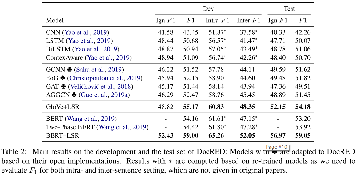
如表2所示,glove的LSR在测试集上达到54.18f1,这是glove模型的最新结果。特别是,我们的模型始终比基于序列的模型有显著的优势。例如,LSR在基于最佳序列的模型BiLSTM上改进了3.1个F1点。这表明直接编码整个文档的模型无法捕捉文档中存在的句间关系。
在相同的设置下,我们的模型始终优于基于静态图或注意机制的基于图的模型。与EoG相比,我们的LSR模型在开发和测试集上分别提高了3.0和2.4倍。我们还对GCNN模型进行了类似的观察,这表明静态文档级图可能无法捕获文档中的复杂交互。LSR产生的动态潜在结构捕获了更丰富的非局部依赖性。此外,LSR的性能也优于GA-T和AGGCN。这从经验上表明,与使用局部注意和自我注意的模型(V eliˇckovi′c等人,2018;Guo等人,2019a)相比,LSR可以诱导更多信息的文档级结构,以更好地进行推理。我们的LSR模型在ignf1设置下也显示出了它的优越性。
此外,基于glove的LSR模型比基于两种BERT模型的LSR模型得到了更好的结果。这从经验上表明,即使不使用强大的上下文编码器,我们的模型也能够捕获远程依赖。继Wang等人(2019)之后,我们利用BERT作为上下文编码器。如表2所示,我们的带有BERT的LSR模型在DocRED上获得了59.05f1的分数,这是一个新的最先进的结果。截至2019年12月9日ACL截止日期,我们在CodaLab记分板上的第一个位置是别名diskorak。
3.4 Intra- and inter-sentence performance
【论文阅读】Reasoning with Latent Structure Refinement for Document-Level Relation Extraction[ACL2020]
原文:https://www.cnblogs.com/Harukaze/p/14368134.html