代码:
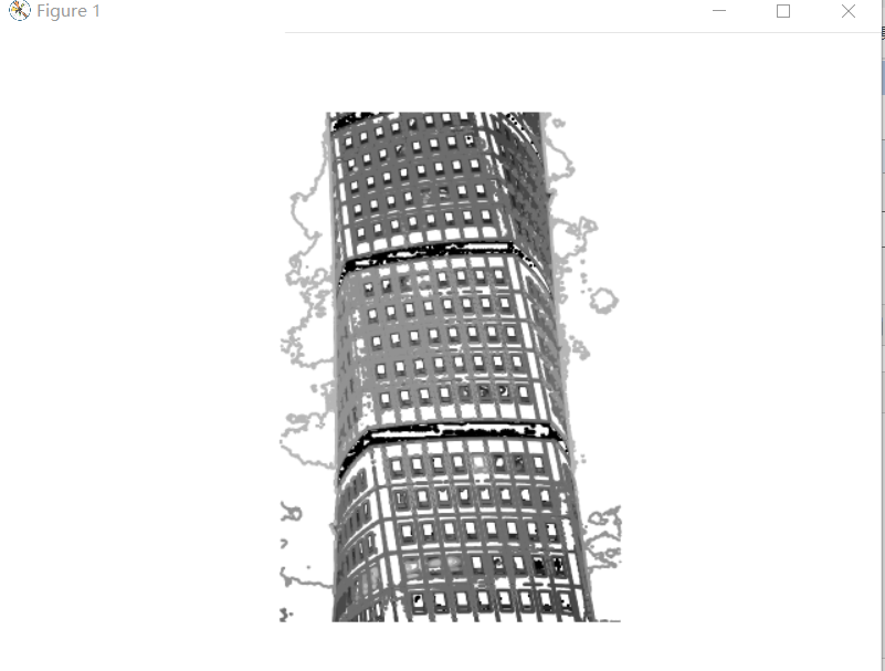
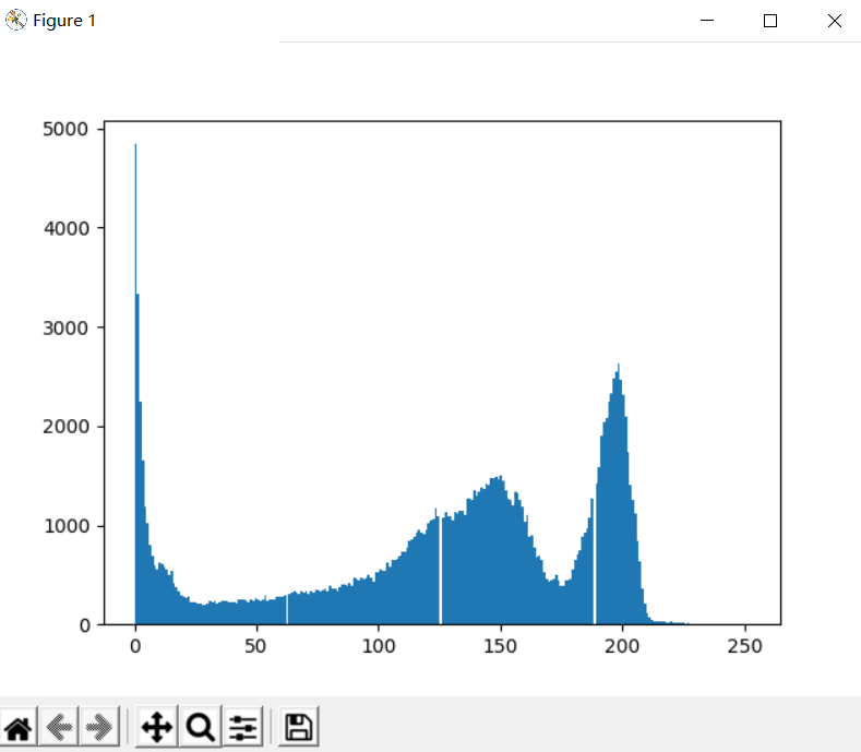
 1 from PIL import Image
 2 from pylab import *
 3
 4 im = array(Image.open(‘2.jpg‘).convert(‘L‘))
 5
 6 figure()
 7 gray()
 8 contour(im,origin=‘image‘)
 9 axis(‘equal‘)
10 axis(‘off‘)
11 figure()
12 hist(im.flatten(),128)
13 show()
使用opencv:
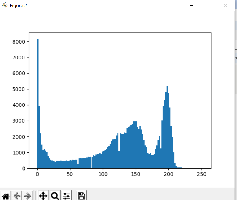
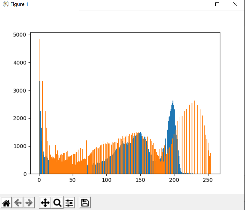
 1 import cv2
 2 from PIL import Image
 3 from numpy import *
 4 from pylab import *
 5
 6 #读取图像
 7 img = cv2.imread(‘2.jpg‘)
 8
 9
10 #创建灰度图像
11 gray = cv2.cvtColor(img,cv2.COLOR_BGR2GRAY)
12
13 figure()
14 hist(gray.ravel(),256)
15 show()
代码:
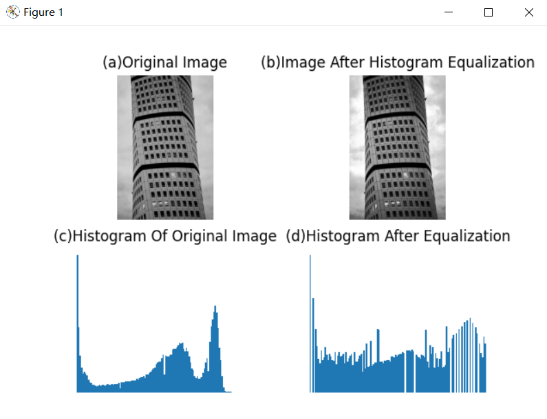
 1 from PIL import Image
 2 from pylab import *
 3 from numpy import *
 4
 5 def histeq(im,nbr_bins=256):
 6
 7   imhist,bins = histogram(im.flatten(),nbr_bins,normed=True)
 8   cdf = imhist.cumsum() # cumulative distribution function
 9   cdf = 255 * cdf / cdf[-1]
10   im2 =interp(im.flatten(),bins[:-1],cdf)
11   return im2.reshape(im.shape),cdf
12
13 im=array(Image.open(‘2.jpg‘).convert(‘L‘))
14 im2,cdf=histeq(im)
15 figure()
16 subplot(2, 2, 1)
17 axis(‘off‘)
18 gray()
19 title(‘(a)Original Image‘)
20 imshow(im)
21
22 subplot(2, 2, 2)
23 axis(‘off‘)
24 title(‘(b)Image After Histogram Equalization‘)
25 imshow(im2)
26
27 subplot(2, 2, 3)
28 axis(‘off‘)
29 title(‘(c)Histogram Of Original Image‘)
30 hist(im.flatten(), 128, density=True)
31
32 subplot(2, 2, 4)
33 axis(‘off‘)
34 title(‘(d)Histogram After Equalization‘)
35 hist(im2.flatten(), 128, density=True)
36
37 show()
使用opencv:
 1 #直方图均衡化
 2
 3 import cv2
 4 from PIL import Image
 5
 6 from pylab import *
 7
 8
 9 img = cv2.imread(‘2.jpg‘)
10
11 gray = cv2.cvtColor(img,cv2.COLOR_BGR2GRAY)
12 cv2.imwrite(‘2gray.jpg‘,gray)
13
14 dst = cv2.equalizeHist(gray)
15
16 # hist_full = cv2.calcHist([dst],[0],None,[256],[0,256])
17 # cv2.imwrite(‘2hist.jpg‘,dst)
18 res = hstack((gray,dst))
19 cv2.imshow("Histogram equalizeHist",res)
20 hist(gray.ravel(),256)
21 hist(dst.ravel(),256)
22 show()
23 cv2.waitKey(0)
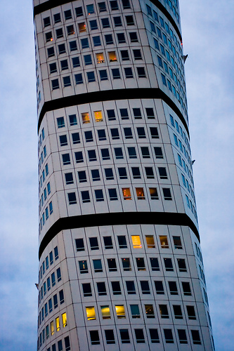
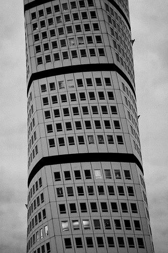
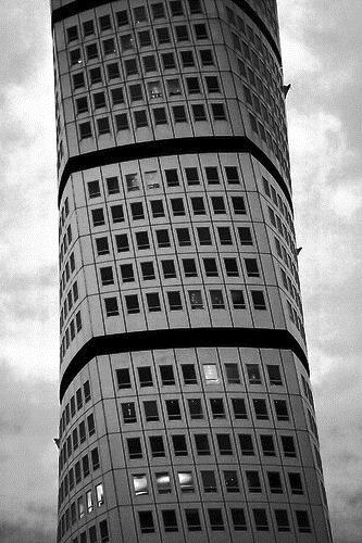
原图 灰度图像 均衡化后
代码:
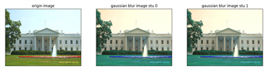
 1 #高斯滤波
 2
 3 import cv2
 4 from pylab import *
 5
 6 def gaussian_blur_func(filename):
 7     img = cv2.imread(filename)
 8     rgbimg = cv2.cvtColor(img,cv2.COLOR_BGR2RGB)
 9     result1 = cv2.GaussianBlur(img,(5,5),0)
10     result2 = cv2.GaussianBlur(img,(5,5),1)
11     titles = [‘origin image‘,‘gaussian blur image stu 0‘,‘gaussian blur image stu 1‘]
12     images = [rgbimg,result1,result2]
13     for i in range(3):
14         subplot(1,3,i+1),imshow(images[i])
15         title(titles[i])
16         xticks([]),yticks([])
17     show()
18
19
20 gaussian_blur_func(‘3.jpg‘)
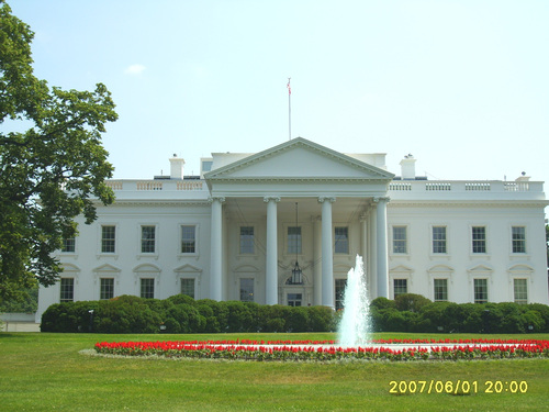
原图
结果
分割线
未完待续...
3/14更
原文:https://www.cnblogs.com/Easy-/p/14503023.html