5.1
Consider the diagrams on the right in Figure 5.1. Why does the estimated value function jump up for the last two rows in the rear? Why does it drop off for the whole last row on the left? Why are the frontmost values higher in the upper diagrams than in the lower?
5.2
Suppose every-visit MC was used instead of first-visit MC on the blackjack task. Would you expect the results to be very different? Why or why not?
5.3
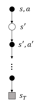
What is the backup diagram for Monte Carlo estimation of \(q_\pi\)?

5.4
The pseudocode for Monte Carlo ES is inefficient because, for each state–action pair, it maintains a list of all returns and repeatedly calculates their mean. It would be more efficient to use techniques similar to those explained in Section 2.4 to maintain just the mean and a count (for each state–action pair) and update them incrementally. Describe how the pseudocode would be altered to achieve this.
5.5
Consider an MDP with a single nonterminal state and a single action that transitions back to the nonterminal state with probability \(p\) and transitions to the terminal state with probability \(1?p\). Let the reward be +1 on all transitions, and let \(\gamma=1\). Suppose you observe one episode that lasts 10 steps, with a return of 10. What are the first-visit and every-visit estimators of the value of the nonterminal state?
5.6 What is the equation analogous to (5.6) for action values \(Q(s, a)\) instead of state values \(V(s)\), again given returns generated using \(b\)?
因为\(q_\pi(s,a)\)已经把\(S_k\)下\(A_k\)选过了,所以只用决定\(t+1\)之后的动作序列。此外,之前定义的\(\mathcal{T}(s)\)是只包含状态的时刻表示,改为包含动作的\(\mathcal{T}(s,a)\),最终有
5.7
In learning curves such as those shown in Figure 5.3 error generally decreases with training, as indeed happened for the ordinary importance-sampling method. But for the weighted importance-sampling method error first increased and then decreased. Why do you think this happened?
5.8
The results with Example 5.5 and shown in Figure 5.4 used a first-visit MC method. Suppose that instead an every-visit MC method was used on the same problem. Would the variance of the estimator still be infinite? Why or why not?
根据上面这个式子,把多次访问的序列拆成every-visit的形式,计算平均。比如长度1的序列不变,长度为2的序列计算两次,长度为3的序列计算3次,以此类推。
所以也是无穷的。
之前我一直在想需不需要平均,是不是加起来就行了。后来觉得,既然是期望,那么去掉ratio和return部分,关于概率的积分应该为1才行,比如every-visit里面每条轨迹出现的概率之和为1。如果不平均,那不是相当于这条轨迹出现的概率增加了,所以还是除以一下把后面的值算到轨迹的平均值里可能更说得通。
5.9
Modify the algorithm for first-visit MC policy evaluation (Section 5.1) to use the incremental implementation for sample averages described in Section 2.4.
5.10
Derive the weighted-average update rule (5.8) from (5.7). Follow the pattern of the derivation of the unweighted rule (2.3).
5.11
In the boxed algorithm for off-policy MC control, you may have been expecting the \(W\) update to have involved the importance-sampling ratio \(\frac{\pi(A_t|S_t)}{b(A_t|S_t)}\), but instead it involves \(\frac{1}{b(A_t|S_t)}\). Why is this nevertheless correct?
5.12:
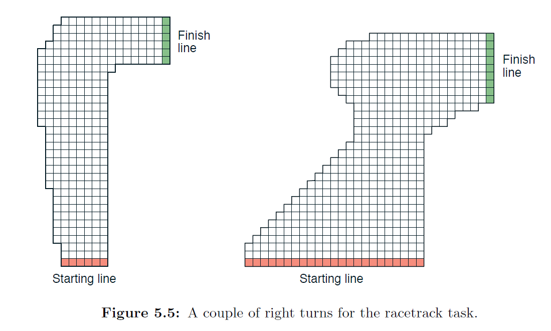
Racetrack (programming) Consider driving a race car around a turn like those shown in Figure 5.5. You want to go as fast as possible, but not so fast as to run off the track. In our simplified racetrack, the car is at one of a discrete set of grid positions, the cells in the diagram. The velocity is also discrete, a number of grid cells moved horizontally and vertically per time step. The actions are increments to the velocity components. Each may be changed by +1, ?1, or 0 in each step, for a total of nine (3x3) actions. Both velocity components are restricted to be nonnegative and less than 5, and they cannot both be zero except at the starting line. Each episode begins in one of the randomly selected start states with both velocity components zero and ends when the car crosses the finish line. The rewards are ?1 for each step until the car crosses the finish line. If the car hits the track boundary, it is moved back to a random position on the starting line, both velocity components are reduced to zero, and the episode continues. Before updating the car’s location at each time step, check to see if the projected path of the car intersects the track boundary. If it intersects the finish line, the episode ends; if it intersects anywhere else, the car is considered to have hit the track boundary and is sent back to the starting line. To make the task more challenging, with probability 0.1 at each time step the velocity increments are both zero, independently of the intended increments. Apply a Monte Carlo control method to this task to compute the optimal policy from each starting state. Exhibit several trajectories following the optimal policy (but turn the noise off for these trajectories).

5.13
Show the steps to derive (5.14) from (5.12).
5.14
Modify the algorithm for off-policy Monte Carlo control (page 111) to use the idea of the truncated weighted-average estimator (5.10). Note that you will first need to convert this equation to action values.
| t | r & b | \(\bar G\) | \(\rho\) | \(\Gamma\) | 结果 G & W |
|---|---|---|---|---|---|
| - | - |
\([0,\cdots,0]\) |
\([0,\cdots,0]\) |
\([0,\cdots,0]\) |
- |
| \(T-1\) | \(R_T\) 1 |
\([0,\cdots,0,\bar G_{T-1:T}]\) | \([0,\cdots,0,1]\) | \([0,\cdots,0,1]\) | \(\bar G_{T-1:T}\) \(1\) |
| \(T-2\) | \(R_{T-1}\) \(b(A_{T-1}\|S_{T-1})\) |
\([\cdots,\bar G_{T-2:T-1},\bar G_{T-2:T}]\) | \([0,\cdots,1,\rho_{T-1:T-1}]\) | \([0,\cdots,1,\gamma]\) | \((1-\gamma)\sum^{T-1}_{h=T-1}\gamma^{h-T+1}\rho_{T-1:h-1}\bar G_{T-2:h}+\gamma \rho_{T-1:T-1}\bar G_{T-1:T})\) \((1-\gamma)\sum^{T-1}_{h=T-1}\gamma^{h-T+1}\rho_{T-1:h-1}+\gamma \rho_{T-1:T-1})\) |
| \(T-3\) | \(R_{T-2}\) \(b(A_{T-2}\|S_{T-2})\) |
\([\cdots,\bar G_{T-3:T-2},\bar G_{T-3:T-1},\bar G_{T-3:T}]\) | \([\cdots,1,\rho_{T-2:T-2},\rho_{T-2:T-1}]\) | \([\cdots,1,\gamma,\gamma^2]\) | \((1-\gamma)\sum^{T-1}_{h=T-2}\gamma^{h-T+2}\rho_{T-2:h-1}\bar G_{T-3:h}+\gamma^{2}\rho_{T-2:T-1}\bar G_{T-3:T})\) \((1-\gamma)\sum^{T-1}_{h=T-2}\gamma^{h-T+2}\rho_{T-2:h-1}+\gamma^{2}\rho_{T-2:T-1})\) |
| ... | ... | ... | ... | ... | ... |
6.1
If \(V\) changes during the episode, then (6.6) only holds approximately; what would the difference be between the two sides? Let \(V_t\) denote the array of state values used at time \(t\) in the TD error (6.5) and in the TD update (6.2). Redo the derivation above to determine the additional amount that must be added to the sum of TD errors in order to equal the Monte Carlo error.
所以\(\delta_t\)都写成和更新时刻\(t\)相关的式子:
题目就是说之前\(\delta_t\)没有区别这个地方,改成这个形式,如下:
6.2
This is an exercise to help develop your intuition about why TD methods are often more efficient than Monte Carlo methods. Consider the driving home example and how it is addressed by TD and Monte Carlo methods. Can you imagine a scenario in which a TD update would be better on average than a Monte Carlo update? Give an example scenario—a description of past experience and a current state—in which you would expect the TD update to be better. Here’s a hint: Suppose you have lots of experience driving home from work. Then you move to a new building and a new parking lot (but you still enter the highway at the same place). Now you are starting to learn predictions for the new building. Can you see why TD updates are likely to be much better, at least initially, in this case? Might the same sort of thing happen in the original scenario?
6.3
From the results shown in the left graph of the random walk example it appears that the first episode results in a change in only \(V(A)\). What does this tell you about what happened on the first episode? Why was only the estimate for this one state changed? By exactly how much was it changed?
对于其他状态,更新为\(V(S_t)\leftarrow V(S_t) + 0.1\cdot[0+ 0.5-0.5]\)值不变。对\(A\)有\(V(A)\leftarrow 0.5 + 0.1\cdot[0+ 0-0.5]=0.45\)。
6.4
The specific results shown in the right graph of the random walk example are dependent on the value of the step-size parameter, \(\alpha\). Do you think the conclusions about which algorithm is better would be affected if a wider range of \(\alpha\) values were used? Is there a different, fixed value of \(\alpha\) at which either algorithm would have performed significantly better than shown? Why or why not?
6.5
In the right graph of the random walk example, the RMS error of the TD method seems to go down and then up again, particularly at high \(\alpha \text{‘s}\). What could have caused this? Do you think this always occurs, or might it be a function of how the approximate value function was initialized?
6.6
In Example 6.2 we stated that the true values for the random walk example
are \(\frac{1}{6},\frac{2}{6},\frac{3}{6},\frac{4}{6},\text{and} \ \frac{5}{6}\), for states A through E. Describe at least two different ways that these could have been computed. Which would you guess we actually used? Why?
则有
直接写出矩阵解出来即可。有代码如下:
	import numpy as np
	P =np.matrix([[0,0,0,0,0,0,0],
	  [0.5,0,0.5,0,0,0,0],
	  [0,0.5,0,0.5,0,0,0],
	  [0, 0,0.5, 0, 0.5, 0, 0],
	  [0, 0, 0,0.5, 0, 0.5, 0],
	  [0,0,0,0,0.5,0,0.5],
	  [0, 0, 0, 0, 0, 0,0]])
	I = np.eye(7)
	R = np.matrix([[0,0,0,0,0,1/2,0.]]).T

	print(np.dot(np.linalg.inv(I-P),R))
得到\([0,\frac{1}{6},\frac{2}{6},\frac{3}{6},\frac{4}{6},\frac{5}{6},0]\)
6.7
Design an off-policy version of the TD(0) update that can be used with arbitrary target policy \(\pi\) and covering behavior policy \(b\), using at each step \(t\) the importance sampling ratio \(\rho_{t:t}\) (5.3).
此时有\(v_\pi(s)=E_{\pi}[G_t|S_t=s]\)。
根据式子(5.4)现在有\(v_\pi(s)=E_b[\rho_{t:T-1}G_t|S_t=s]\),其中数据来自\(b\)。所以要做的事情就是把\(G_t\)换成\(\rho_{t:T-1}G_t\),所以(6.1)有\(V(S_t)\leftarrow V(S_t)+\alpha [\rho_{t:T-1}G_t-V(S_t)]\)。另一方面
所以(6.2)有\(V(S_t)\leftarrow V(S_t)+\alpha [\rho_{t:t}R_{t+1}+ \rho_{t:t}\gamma V(S_{t+1})-V(S_t)]\),即带重要性采样的TD(0)更新。
6.8
Show that an action-value version of (6.6) holds for the action-value form of the TD error (\(\delta_t =R_{t+1}+\gamma Q(S_{t+1},A_{t+1})-Q(S_t,A_t)\), again assuming that the values don’t change from step to step.
6.9:
Windy Gridworld with King’s Moves (programming) Re-solve the windy gridworld assuming eight possible actions, including the diagonal moves, rather than the usual four. How much better can you do with the extra actions? Can you do even better by including a ninth action that causes no movement at all other than that caused by the wind?
6.10:
Stochastic Wind (programming) Re-solve the windy gridworld task with King’s moves, assuming that the effect of the wind, if there is any, is stochastic, sometimes varying by 1 from the mean values given for each column. That is, a third of the time you move exactly according to these values, as in the previous exercise, but also a third of the time you move one cell above that, and another third of the time you move one cell below that. For example, if you are one cell to the right of the goal and you move left, then one-third of the time you move one cell above the goal, one-third of the time you move two cells above the goal, and one-third of the time you move to the goal.
6.11
Why is Q-learning considered an off-policy control method?
6.12 Suppose action selection is greedy. Is Q-learning then exactly the same algorithm as Sarsa? Will they make exactly the same action selections and weight updates?
6.13
What are the update equations for Double Expected Sarsa with an \(\epsilon\)-greedy target policy?
把Q换成两个,
其中\(\pi(a|S_t)= \left\{\begin{array}{l} 1-\epsilon+\epsilon/|\mathcal{A}(S_t)|, \quad if \ a=A^*\\epsilon/|\mathcal{A}(S_t)|, \qquad \qquad \ if \ a \not = A^* \end{array}\right.\)
6.14
Describe how the task of Jack’s Car Rental (Example 4.2) could be reformulated in terms of afterstates. Why, in terms of this specific task, would such a reformulation be likely to speed convergence?
原文:https://www.cnblogs.com/initial-h/p/14811709.html