We use mean cross entropy loss, because it is good for multi-category problems;
We use ReLu as activation function due to excellent adaptability to multi-class classification. We have also tested sigmoid, but there are problems with vanishing gradients.
The input layer has 784 neurons, because the count of pixel is \(28 \times 28\);
The output layer has 10 neurons, because we need to classify 10 categories.
The selection strategy of learning rate is constantly changing in the process of network training. At the beginning, the parameters are relatively random, so we should choose a relatively large learning rate, so that loss will fall faster. When we train for a period of time, the parameter update should have a smaller range of change, and then we choose a smaller learning rate
Full code is below:
import numpy as np
from matplotlib import pyplot as plt
def initialize(hidden_dim, output_dim):
# retrieve mnist data
X_train = np.loadtxt(‘./dataSets/mnist_small_train_in.txt‘, delimiter=‘,‘)
X_test = np.loadtxt(‘./dataSets/mnist_small_test_in.txt‘, delimiter=‘,‘)
y_train = np.loadtxt(‘./dataSets/mnist_small_train_out.txt‘, delimiter=‘,‘, dtype="int32")
y_test = np.loadtxt(‘./dataSets/mnist_small_test_out.txt‘, delimiter=‘,‘, dtype="int32")
# normalize data
X_train = (X_train - np.mean(X_train)) / np.std(X_train)
X_test = (X_test - np.mean(X_test)) / np.std(X_test)
# one hot encode labels
temp_y_train = np.eye(10)[y_train]
temp_y_test = np.eye(10)[y_test]
y_train = temp_y_train.reshape(list(y_train.shape) + [10])
y_test = temp_y_test.reshape(list(y_test.shape) + [10])
# weights for single hidden layer
W1 = np.random.randn(hidden_dim, X_train.shape[1]) * 0.01
b1 = np.zeros((hidden_dim,))
W2 = np.random.randn(output_dim, hidden_dim) * 0.01
b2 = np.zeros((output_dim,))
parameters = [W1, b1, W2, b2]
# return to column vectors
return parameters, X_train.T, X_test.T, y_train.T, y_test.T
def sigmoid(x):
return 1.0 / (1.0 + np.exp(-x))
def dsigmoid(x):
# input x is already sigmoid, no need to recompute
return x * (1.0 - x)
def ReLU(x):
return x * (x > 0)
def dReLU(x):
return 1. * (x > 0)
# Cross entropy loss
def closs(pred, y):
return np.squeeze(-np.sum(np.multiply(np.log(pred), y)) / len(y))
def dcloss(pred, y):
return pred - y
# Mean squared error loss
def loss(pred, y):
return np.sum(.5 * np.sum((pred - y) ** 2, axis=0), axis=0) / y.shape[1]
def dloss(pred, y):
return (pred - y) / y.shape[1]
class NeuralNet(object):
def __init__(self, hidden_dim, output_dim):
# size of layers
self.hidden_dim_1 = hidden_dim
self.output_dim = output_dim
# weights and data
parameters, self.x_train, self.x_test, self.y_train, self.y_test = initialize(hidden_dim, output_dim)
self.W1, self.b1, self.W2, self.b2 = parameters
# activations
batch_size = self.x_train.shape[0]
self.ai = np.ones((self.x_train.shape[1], batch_size))
self.ah1 = np.ones((self.hidden_dim_1, batch_size))
self.ao = np.ones((self.output_dim, batch_size))
# classification output for transformed OHE
self.classification = np.ones(self.ao.shape)
# container for loss progress
self.loss = None
self.test_error = None
def forward_pass(self, x):
# input activations
self.ai = x
# hidden_1 activations
self.ah1 = sigmoid(self.W1 @ self.ai + self.b1[:, np.newaxis])
# output activations
self.ao = sigmoid(self.W2 @ self.ah1 + self.b2[:, np.newaxis])
# transform to OHE for classification
self.classification = (self.ao == self.ao.max(axis=0, keepdims=0)).astype(float)
def backward_pass(self, target):
# calculate error for output
out_error = dloss(self.ao, target)
out_delta = out_error * dsigmoid(self.ao)
# calculate error for hidden_1
hidden_1_error = self.W2.T @ out_delta
hidden_1_delta = hidden_1_error * dReLU(self.ah1)
# derivative for W2/b2 (hidden_1 --> out)
w2_deriv = out_delta @ self.ah1.T
b2_deriv = np.sum(out_delta, axis=1)
# derivative for W1/b1 (input --> hidden_1)
w1_deriv = hidden_1_delta @ self.ai.T
b1_deriv = np.sum(hidden_1_delta, axis=1)
return [w1_deriv, b1_deriv, w2_deriv, b2_deriv]
def train(self, epochs, lr, batch_size=128):
self.loss = np.zeros((epochs,))
self.test_error = np.zeros((epochs,))
for epoch in range(epochs):
indices = np.arange(self.x_train.shape[1])
np.random.shuffle(indices)
for i in range(0, self.x_train.shape[1] - batch_size + 1, batch_size):
excerpt = indices[i:i + batch_size]
batch_x, batch_y = self.x_train[:, excerpt], self.y_train[:, excerpt]
# compute output of forward pass
self.forward_pass(batch_x)
# back prop error
w1_deriv, b1_deriv, w2_deriv, b2_deriv = self.backward_pass(batch_y)
# adjust weights with simple SGD
self.W1 -= lr * w1_deriv
self.b1 -= lr * b1_deriv
self.W2 -= lr * w2_deriv
self.b2 -= lr * b2_deriv
# compute error
self.forward_pass(self.x_test)
error = loss(self.ao, self.y_test)
self.loss[epoch] = error
t = 0
for i, pred in enumerate(self.classification.T):
if np.argmax(self.y_test.T[i]) == np.argmax(pred):
t += 1
acc = t / self.classification.shape[1]
self.test_error[epoch] = 1 - acc
# print progress
if (epoch + 1) % 50 == 0:
print("Epoch {}/{} -> loss: {:.5f} -> val_acc: {:.5f}".format(epoch + 1, epochs, error, acc))
def predict(self, x):
self.forward_pass(x)
return self.classification
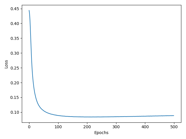
def visualize_prediction(self, expected, predicted):
# plot loss progress
plt.figure(2)
plt.plot(self.loss)
plt.xlabel("Epochs")
plt.ylabel("Loss")
plt.show()
# plot loss progress
plt.figure(3)
plt.plot(self.test_error)
plt.xlabel("Epochs")
plt.ylabel("Test Error")
plt.show()
nn = NeuralNet(hidden_dim=784, output_dim=10)
nn.train(epochs=500, lr=.05)
y_hat = nn.predict(nn.x_test)
t = 0
for i, pred in enumerate(y_hat.T):
if np.argmax(nn.y_test.T[i]) == np.argmax(pred):
t += 1
print("Accuracy:", t / y_hat.shape[1])
nn.visualize_prediction(nn.y_test.T, y_hat.T)
Show how the misclassification error (in percent) on the testing set evolves during learning:

Full code is below:
import numpy as np
from matplotlib import pyplot as plt
def target(x):
s = np.sin(x)
return s + np.square(s)
def kernel(x, z):
return np.exp(-(x - z) ** 2)
def compute_c(x, noise):
return kernel(x, x) + noise
def predict(x, X, Y, C_inv, noise):
k = np.array([kernel(x, val) for val in X])
mean = k.T.dot(C_inv).dot(Y)
std = np.sqrt(compute_c(x, noise) - k.T.dot(C_inv).dot(k))
return mean, std
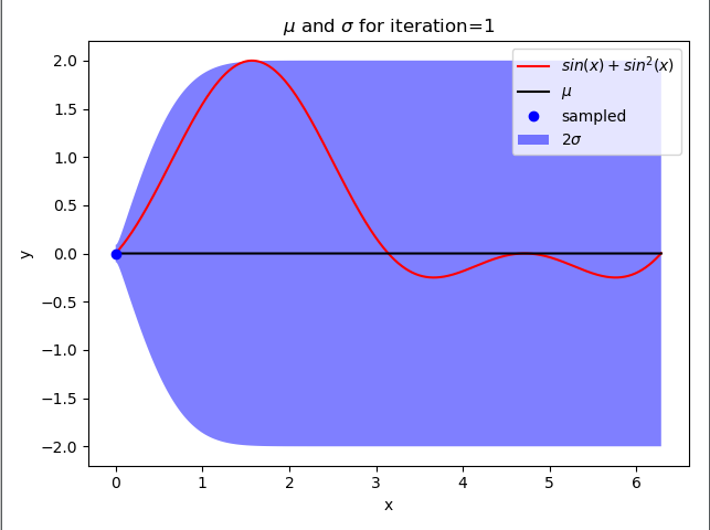
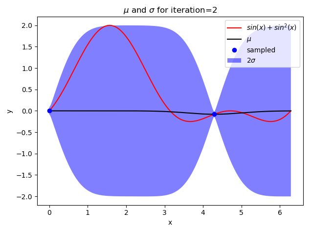
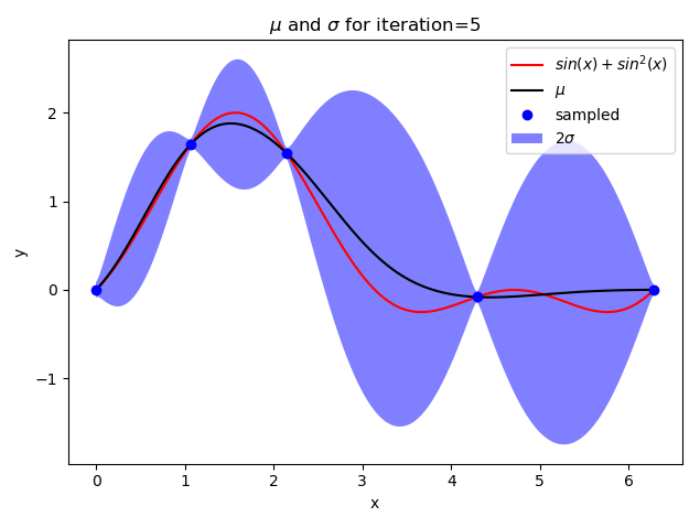
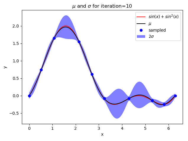
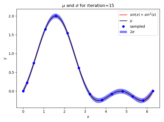
def plot_gp(X, mean, std, iteration):
y1 = mean - 2 * std
y2 = mean + 2 * std
plt.plot(X, target(X), "-", color="red", label="$sin(x) + sin^2(x)$")
plt.plot(X, mean, color="black", label="$\mu$")
plt.fill_between(X, y1, y2, facecolor=‘blue‘, interpolate=True, alpha=.5, label="$2\sigma$")
plt.title("$\mu$ and $\sigma$ for iteration={}".format(iteration))
plt.xlabel("x")
plt.ylabel("y")
def gpr():
noise = 0.001
step_size = 0.005
X = np.arange(0, 2 * np.pi + step_size, step_size)
iterations = 15
std = np.array([np.sqrt(compute_c(x, noise)) for x in X])
j = np.argmax(std)
Xn = np.array([X[j]])
Yn = np.array([target(Xn)])
C = np.array(compute_c(X[j], noise)).reshape((1, 1))
C_inv = np.linalg.solve(C, np.identity(C.shape[0]))
for iteration in range(0, iterations):
mean = np.zeros(X.shape[0])
std = np.zeros(X.shape[0])
for i, x in enumerate(X):
mean[i], std[i] = predict(x, Xn, Yn, C_inv, noise)
if iteration + 1 in [1, 2, 5, 10, 15]:
plot_gp(X, mean, std, iteration + 1)
plt.plot(Xn, Yn, "o", c="blue", label="sampled")
plt.legend()
plt.show()
j = np.argmax(std)
Xn = np.append(Xn, X[j])
Yn = np.append(Yn, target(Xn[-1]))
# update C matrix
x_new = Xn[-1]
k = np.array([kernel(x_new, val) for val in Xn])
c = kernel(x_new, x_new) + noise
dim = C.shape[0]
C_new = np.empty((dim + 1, dim + 1))
C_new[:-1, :-1] = C
C_new[-1, -1] = c
C_new[:, -1] = k
C_new[-1:] = k.T
C = C_new
C_inv = np.linalg.solve(C, np.identity(C.shape[0]))
gpr()
原文:https://www.cnblogs.com/Java-Starter/p/15096534.html