Notes Berkerly Statistics 2.1X Week4

We’ve studied distributionin histogram , measures of location/ spread. range. and more for normaldistributions.

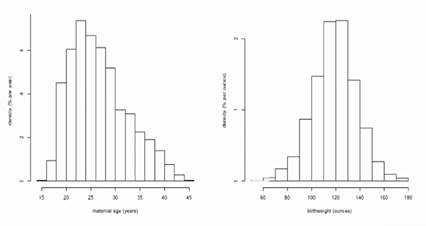
we start by looking at twovariable , start from histogram analysis.

univariate data

Bivariate data : scatterdiagram

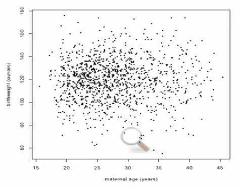
cant see relation

 ( scatter. As in Octave )

Bivariate data : positiveassociation , linear

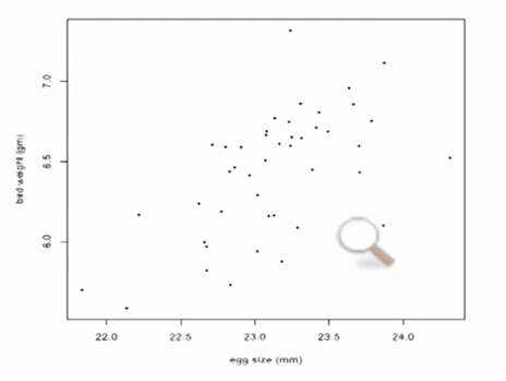
association : any relation between variables.

positive association: above average values of onevariable tend to go with the above average values of the other; the scatterslopes up

and corresponding to negative association

linear association : roughly , the scatter diagram is clustered around a straight line.

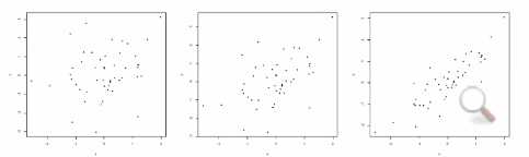
Football-shaped scatterplot[橄榄球]

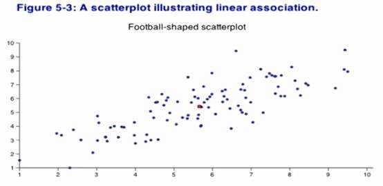
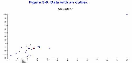
May lay out with outlier

for the same scale, wecould see how linear two variables are

correlationcoefficient ( r ) : a number to discribe how linear a set of data is.

Intuition

could see the correspondngdirections from mean of xs and ys.

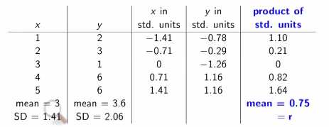
Formula

1. convert both lists instd.units.

2. multiply from thecorrespoding position

3. mean of products.

Math

r = 1/n *SUM( ( stdx ) * (stdy) )

Properties of r

1. a pure number.

2. -1<=r<=1 ,intuition : the mean of the products in the std.units.

3. switch the variables x,y, r stays the same.

for linear transformations:

4. add a constant to onethe of lists , r stays the same , u know.

5. multiplying one thelists by a positive constant does not change standard units , ( think , as howto measure , or using different units for data.) , so r stays 

6. and for a negativemultiplier ?~ u can imagine!

R makes the degreeof the linear associations.~

think of the bigger shoes of children wearingon , the more ability of reading to them !

( the basic statistical principle! )

if two variables have anon-zero correlation, they are related to each other in some way , but doesn‘tmean that one is the cause of the other!

correlated : linearlyrelation.

one point , noticableeffect on r , for a outlier

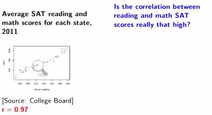
consider , knowing twovariables are linear associated , and knowing the correlation .

can u estimate another fromone of the known variable data. ==> Regression ,u know how important it is.

Estimate: one variable

Heights: average 67 inches,SD 3inches.

so , one of these people ispicked, u have to estimate the person‘s height.

so , u guess 67 inches.

error : actual height - 67inches = actual height - average height.

error in using the averageas the estimate : deviation from average

rough size of errors = r.m.s of deviation from average = SD = 3 inches.

chebychev: For at least 75% of the people , the estimate will be correct to within 6inches.

and if roughly normal distribution , 95% , will be correct to within 6 inches.

makes the smallest error.

THE r.m.s of the errorswill be smallest if u choose c = average

average: least squaresestimate

Given the values of onevariable , and estimate the other.

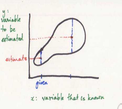
Regression line: intuition; the equation in standards units; regression estimates.

How to identify the best line- > Equation of the regression line

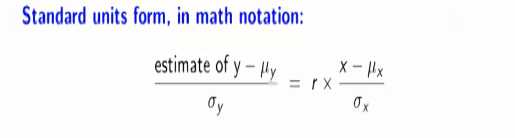
estimate y = r*x given x ,correlation r.

in standard units of y,x

SO WHY , CAN U INTUIT IT ?

1.Heights: average 67inches, SD 3 inches.

Weights : average 160pounds , SD 20 pounds.

r = 0.6

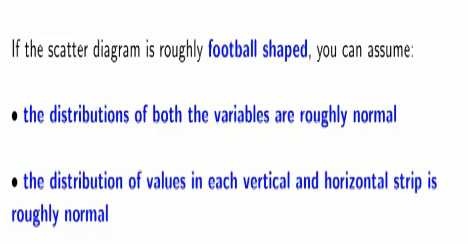
scatter diagram is roughlyfootball shaped.

Estimate a person with 73inches may weigh how many pounds ?

73 inches in standard units= (73-67)/3 = 2

estimate of weight instandard units = 2*0.6 = 1.2

so estimate of weight inpound = 1.2 * 20 + 160 = 184 pounds.

2.Midterm and final coursesin a large class have a correlation of 0.5 .

The scatter diagram is roughlyfootball shaped.

One of the students is onthe 80th percentile of midterm scores. Estimate the students‘ percentile rankon the final.

so ,using football shapedproperty: roughly normal.

Sir Francis Galton , 1822 –1911 , given the following terminology first:

SD

correlation

regression

Galton‘s observation:Fathers who are tall tend to have sons who are note quite that tall , onaverage.

we saw that forfootball-shaped scatterplots the graph of averages is not as steep as the SD line, unless r=±1: If 0<r<1, the average value of Y for individuals whose values of X areabout kSDX above the mean(X) is less than kSDY above themean(Y). Similarly, if ?1<r<0,the average value of Y for individuals whose values of X are about kSDX abovemean(X) is less than kSDY below mean(Y).

This phenomenon is calledthe regression effect or regression towards the mean.

Individualswith a given value of X tend to have values of Y that are closer to themean, where closer means fewer SD away.

Thealgebra is correct. The phenomenon is quitegeneral. It is called the regressioneffect. The regression effect is caused bythe same thing that makes the slope of the regression line smaller inmagnitude than the slope of the SD line. If the scatterplot is football-shaped and r is at leastzero but less than 1, then

In a vertical slicecontaining above-average values of X, most of the y coordinates are below theSD line.

In a vertical slicecontaining below-average values of X, most of the y coordinates are above theSD line.

SOURCE

this is confusing for me right now , maybe later , i shouldread it again.

but i understand the general meaning of the regressioneffect , that is the estimate performs more to the average .

slope = r*sigmay/ sigmax ;intercept = mu y - slope * mu * x

use the slope equation tocalculate more conveniently.

"Plug in" mu x asthe value of x.

estimateof y = mu y  ==> the regression line passes through the point ofaverages.

the data meaning , a grouppeople measured at the same time period.