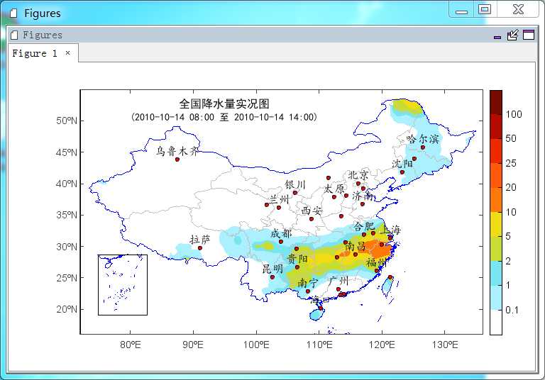
站点数据绘制等值线需要首先将站点数据插值为格点数据,MeteoInfo中提供了反距离权法(IDW)和cressman两个方法,其中IDW方法可以有插值半径的选项。这里示例读取一个MICAPS第一类数据(地面全要素观测),获取6小时累积降水数据(Precipitation6h),然后用站点数据的griddata函数将站点数据插值为格点数据,再利用contourfm函数创建等值线填色图层(等值线间隔和颜色可以自定义)。
脚本程序(经纬度投影):
#Set data folders
basedir = ‘D:/MyProgram/Distribution/java/MeteoInfo/MeteoInfo‘
datadir = os.path.join(basedir, ‘sample/MICAPS‘)
mapdir = os.path.join(basedir, ‘map‘)
#Read shape files
bou2_layer = shaperead(os.path.join(mapdir, ‘bou2_4p.shp‘))
bou1_layer = shaperead(os.path.join(mapdir, ‘bou1_4l.shp‘))
china_layer = shaperead(os.path.join(mapdir, ‘china.shp‘))
city_layer = shaperead(os.path.join(mapdir, ‘res1_4m.shp‘))
#Read station data
f = addfile_micaps(os.path.join(datadir, ‘10101414.000‘))
pr = f.stationdata(‘Precipitation6h‘)
#griddata function - interpolate
x = arange(75, 135, 0.5)
y = arange(18, 55, 0.5)
prg = pr.griddata((x, y), method=‘idw‘, radius=3)
#Plot
axesm()
geoshow(bou2_layer, edgecolor=‘lightgray‘)
geoshow(bou1_layer, facecolor=(0,0,255))
geoshow(city_layer, facecolor=‘r‘, size=4, labelfield=‘NAME‘, fontname=u‘楷体‘, fontsize=16, yoffset=15)
geoshow(china_layer, visible=False)
levs = [0.1, 1, 2, 5, 10, 20, 25, 50, 100]
cols = [(255,255,255),(170,240,255),(120,230,240),(200,220,50),(240,220,20),(255,120,10),(255,90,10),     (240,40,0),(180,10,0),(120,10,0)]
layer = contourfm(prg, levs, colors=cols)
masklayer(china_layer, [layer])
colorbar(layer)
xlim(72, 136)
ylim(16, 55)
text(95, 52, u‘全国降水量实况图‘, fontname=u‘黑体‘, fontsize=16)
text(95, 50, u‘(2010-10-14 08:00 至 2010-10-14 14:00)‘, fontname=u‘黑体‘, fontsize=14)
#Add south China Sea
sc_layer = bou1_layer.clone()
axesm(position=[0.14,0.18,0.15,0.2], axison=False)
geoshow(sc_layer, facecolor=(0,0,255))
xlim(106, 123)
ylim(2, 23)
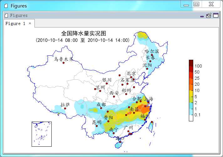
脚本程序(Lambert投影):
#Set data folders
basedir = ‘D:/MyProgram/Distribution/java/MeteoInfo/MeteoInfo‘
datadir = os.path.join(basedir, ‘sample/MICAPS‘)
mapdir = os.path.join(basedir, ‘map‘)
#Read shape files
bou2_layer = shaperead(os.path.join(mapdir, ‘bou2_4p.shp‘))
bou1_layer = shaperead(os.path.join(mapdir, ‘bou1_4l.shp‘))
china_layer = shaperead(os.path.join(mapdir, ‘china.shp‘))
city_layer = shaperead(os.path.join(mapdir, ‘res1_4m.shp‘))
#Read station data
f = addfile_micaps(os.path.join(datadir, ‘10101414.000‘))
pr = f.stationdata(‘Precipitation6h‘)
#griddata function - interpolate
x = arange(75, 135, 0.5)
y = arange(18, 55, 0.5)
prg = pr.griddata((x, y), method=‘idw‘, radius=3)
#Plot
proj = projinfo(proj=‘lcc‘, lon_0=105, lat_1=25, lat_2=47)
axesm(projinfo=proj, position=[0, 0, 0.9, 1], axison=False, gridlabel=False, frameon=False)
geoshow(bou2_layer, edgecolor=‘lightgray‘)
geoshow(bou1_layer, facecolor=(0,0,255))
geoshow(city_layer, facecolor=‘r‘, size=4, labelfield=‘NAME‘, fontname=u‘楷体‘, fontsize=16, yoffset=15)
geoshow(china_layer, visible=False)
levs = [0.1, 1, 2, 5, 10, 20, 25, 50, 100]
cols = [(255,255,255),(170,240,255),(120,230,240),(200,220,50),(240,220,20),(255,120,10),(255,90,10),     (240,40,0),(180,10,0),(120,10,0)]
layer = contourfm(prg, levs, colors=cols)
masklayer(china_layer, [layer])
colorbar(layer, shrink=0.5, aspect=15)
axism([78, 130, 14, 53])
text(95, 53, u‘全国降水量实况图‘, fontname=u‘黑体‘, fontsize=18)
text(95, 51, u‘(2010-10-14 08:00 至 2010-10-14 14:00)‘, fontname=u‘黑体‘, fontsize=16)
#Add south China Sea
sc_layer = bou1_layer.clone()
axesm(position=[0.1,0.05,0.15,0.2], axison=False)
geoshow(sc_layer, facecolor=(0,0,255))
xlim(106, 123)
ylim(2, 23)
运行结果:
原文:http://www.cnblogs.com/yaqiang/p/4609849.html